library(tidyverse)
survey <- read_csv("https://raw.githubusercontent.com/cobriant/teaching-datasets/refs/heads/main/survey.csv")6.4 Hierarchical Clustering
Overview
Unlike k-means clustering, hierarchical clustering does not require specifying the number of clusters beforehand. Instead, it produces a tree-like visualization called a dendrogram, which illustrates how observations are grouped based on similarity.
Data
The analysis uses a simulated survey dataset containing the following variables:
- income: Annual income in dollars
- frequency: Number of shopping trips per month
- enjoyment: Agreement level (0-7) with “Shopping is fun”
- budgetconcern: Agreement level (0-7) with “Shopping is bad for your budget”
- outing: Agreement level (0-7) with “I combine shopping with eating out”
- thriftiness: Agreement level (0-7) with “I try to get the best buys while shopping”
Visualizations
Explore this data set and create 3 visualizations using ggplot.
Hierarchical Clustering Process
Each leaf in the dendrogram represents an observation, and branches form by fusing the most similar observations first. Clusters are determined by making a horizontal cut across the dendrogram, allowing flexibility in choosing the number of clusters.
Creating 4 clusters, what are the most important features of each cluster?
hc.complete <- hclust(dist(survey), method = "complete")

plot(hc.complete)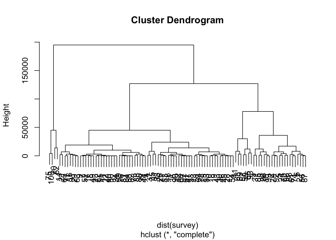
survey %>%
  mutate(cluster = cutree(hc.complete, 4))
# A tibble: 100 × 7
income frequency enjoyment budgetconcern outing thriftiness cluster
<dbl> <dbl> <dbl> <dbl> <dbl> <dbl> <int>
1 33000 10 3 4 0 7 1
2 69000 5 3 1 3 0 2
3 103000 8 3 0 2 4 2
4 19000 5 2 7 0 3 1
5 74000 4 2 3 4 7 2
6 77000 8 4 1 4 2 2
7 45000 4 4 4 7 0 1
8 46000 8 4 7 0 5 1
9 45000 9 2 3 1 4 1
10 38000 7 0 6 2 3 1
# ℹ 90 more rowsHierarchical Clustering Algorithm
Hierarchical clustering begins by treating each observation as its own cluster and iteratively merging the closest two clusters, repeating until there’s just one big cluster. Different linkage methods define “distance” between clusters:
- Using cluster centroids: can lead to an undesirable inversion. That is, two clusters get fused at a height below either of the individual clusters, leading to difficulties in visualization and interpretation.
- Complete linkage: compute all pairwise dissimilarities between the observations in cluster A and the observations in cluster B, and record the largest of these dissimilarities.
- Average linkage: compute all pairwise dissimilarities between the observations in cluster A and the observations in cluster B, and record the average of these dissimilarities.
- Single linkage: compute all pairwise dissimilarities between the observations in cluster A and the observations in cluster B, and record the minimum of these dissimilarities.
Scaling Variables
The variables in our data set are measured in very different scales. Because income differs so much compared with the other variables, differences in income will dominate the clustering. It is therefore important to scale the variables so that each variable is weighted equally in the clustering.
Scale variables so that each variable has mean 0 and standard deviation 1, and draw the dendrogram again. Create 4 clusters: what makes each cluster different?