# probs <- c(___)
# sum(probs)
# sum(probs * 0:4)2.1 Probability Review
A random variable is any variable whose value cannot be predicted exactly. A few examples:
- The message you get in a fortune cookie is a random variable.
- The time you spend searching for your keys after you’ve misplaced them is a random variable.
- The number of customers who enter a small retail store on a given day is a random variable.
Some random variables are discrete while others are continuous. What’s the difference? Discrete random variables are counted like the number of M&M’s you have, while continuous random variables are measured like how heavy your bag of candy is. Discrete random variables take on a small number of possible values, while continuous random variables can take on an infinite number of possible values.
Exercise 1: Which of these might be best modeled as discrete?
- The number of likes you get on a social media post
- The weight of a truck
- The number of customers who enter a small retail store on a given day
- The height of a child
- The speed of a train
Answers:
Exercise 2: Let X be the random variable “the number of likes you get on a social media post”. Suppose that you get 0-4 likes per post each with equal probability. Fill out Table 9.1 below.
| \(x_i\) | 0 | 1 | 2 | 3 | 4 |
|---|---|---|---|---|---|
| \(p_i\) | __ | __ | __ | __ | __ |
Answers:
| \(x_i\) | 0 | 1 | 2 | 3 | 4 |
|---|---|---|---|---|---|
| \(p_i\) |
Exercise 3: Continuing from exercise 2, calculate the expected number of likes you get on a social media post \(E[X]\).
Answer:
\(E[x_i] = \sum_i x_i p_i =\)
Exercise 4: Consider the discrete random variable \(X\), which represents “the number of customers who enter a retail store each hour”. The possible values for \(X\) range from 0 to 4 customers. The probabilities follow a halving pattern: if we let \(p_0 = \frac{16}{31}\) be the probability that 0 customers enter, then \(p_1 = \frac{p_0}{2}\) is the probability that 1 customer enters, \(p_2 = \frac{p_1}{2}\) is the probability that 2 customers enter, and so on. First, verify that these probabilities sum to 1. Second, calculate the expected number of customers who enter the store each hour, \(E[X]\). Solve this by using vectors in R.
Answer:
Expected Value Rules
Here are some math rules about the way expected values work. Let \(X\), \(Y\), and \(Z\) be random variables and let \(b\) be a constant.
The expectation of the sum of several random variables is the sum of their expectations: \(E[X + Y + Z] = E[X] + E[Y] + E[Z]\).
Constants can pass outside of an expectation: \(E[bX] = b E[X]\)
The expected value of a constant is that constant: \(E[b] = b\).
Example: Let \(X\) and \(Y\) be random variables and let \(b_1\) and \(b_2\) be consants. If \(Y = b_1 + b_2 X\), then since \(E[Y] = E[b_1 + b_2 X]\), we can simplify using the rules above to get: \(E[Y] = b_1 + b_2 E[X]\).
Exercise 5: Let \(X\) be a random variable and suppose \(E[X] = 3\). If \(Y = 3 + 5 X\), what is \(E[Y]\)?
Answer: \[\begin{align} E[Y] &= E[3 + 5 X] \\ &= \end{align}\]
Variance
The variance of a random variable measures its dispersion: it asks “on average, how far is the variable from its average”? Differences are squared to get rid of the negative sign and punish large deviances a little more. We’ll reserve the greek letter pronounced “sigma” \(\sigma\) for variance (\(\sigma^2\)) and standard deviation (\(\sigma\)). The formula:
\[\begin{align} Var(X) = \sigma_X^2 &= E\left[(X - E[X])^2\right]\\ &= (x_1 - E[X])^2 p_1 + (x_2 - E[X])^2 p_2 + ... + (x_n - E[X])^2 p_n\\ &= \sum_{i = 1}^n (x_i - E[X])^2 p_i \end{align}\]
Notice that because of the square and the fact that probabilities \(p_i\) are never negative, the variance of a random variable can never be a negative number.
Example: Let \(X\) be a dice roll. Then to find \(Var(X)\), recall that we already calculated \(E[X] = 3.5\), so: \[\begin{align} Var(X) &= E[(X - 3.5)^2]\\ &= \frac{1}{6} (1 - 3.5)^2 + \frac{1}{6} (2 - 3.5)^2 + \frac{1}{6} (3 - 3.5)^2 + \\ &\hspace{.7cm} \frac{1}{6} (4 - 3.5)^2 + \frac{1}{6} (5 - 3.5)^2 + \frac{1}{6} (6 - 3.5)^2 \\ &= \frac{17.5}{6} \\ &\approx 2.9167 \end{align}\] This is a measure of the dispersion of a dice roll.
Exercise 6: Again let \(X\) be the random variable “the number of likes you get on a social media post” where you get 0-4 likes per post each with equal probability. What is the variance of \(X\)?
Answer:
\(Var(X) = E[(X - 2)^2] = \sum_i (x_i - 2)^2 p_i\) =
Variance Rules
Here are some rules about the way variance works. Let \(X\) and \(Y\) be random variables and let \(b\) be a constant.
The variance of the sum of two random variables is the sum of their variances plus two times their covariance: \(Var(X + Y) = Var(X) + Var(Y) + 2 Cov(X, Y)\)
Constants that are multiplied can pass outside of a variance if you square them: \(Var(bX) = b^2 Var(X)\)
The variance of a constant is 0: \(Var(b) = 0\).
The variance of a random variable plus a constant is just the variance of that random variable: \(Var(X + b) = Var(X)\).
Exercise 7: Let \(X\) be a random variable and suppose \(Var(X) = 3\). If \(Y = 3 + 5 X\), what is \(Var(Y)\)?
Answer: \[\begin{align} Var(Y) &= Var(3 + 5 X)\\ &= \end{align}\]
Continuous Random Variables
When the variable can take on an infinite number of possible values, the probability it takes on any given value must be zero. So for continuous random variables, we use probability density functions (PDF) and we talk about the probability the random variable lies within an interval.
For example, suppose that the “time spent searching for your keys” is a continuous random variable with uniform probability between 0 and 5 minutes. Figure 9.1 illustrates the PDF: since the area under the PDF must be 1, we know that the height of the rectangle is 1/5.
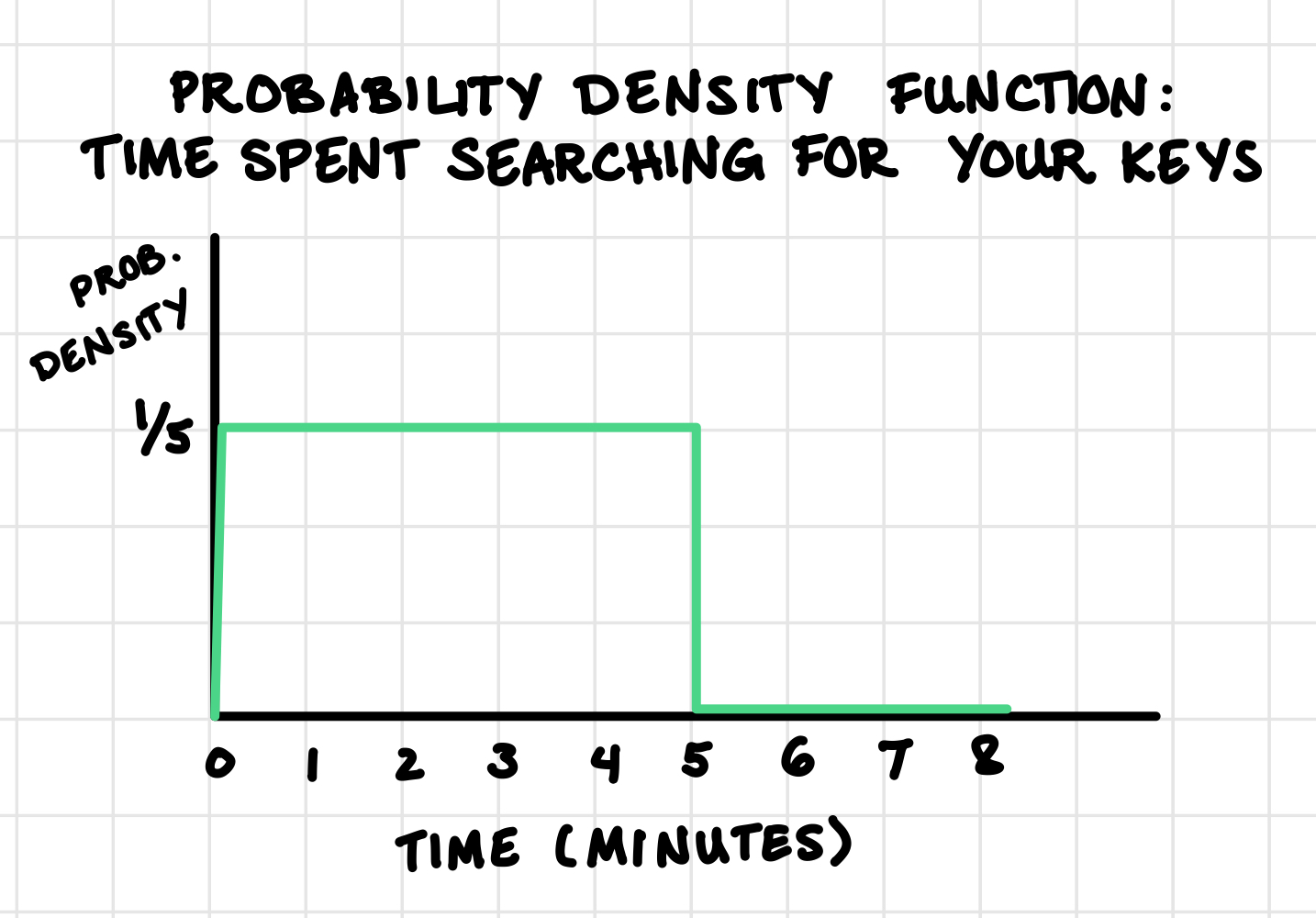
Example: In the example above in Figure 9.1, the probability that you spend less than 1 minute searching for your keys is \(1 \times \frac{1}{5} = 0.20\).
Exercise 8: In Figure 9.1, what is the probability you spend 3 minutes or more searching for your keys?
Answer:
To find the expected value or variance of a continuous random variable instead of a discrete random variable, just swap out integrals for sums and the PDF \(f(X)\) for \(p_i\):
| \(E[X]\) | \(Var(X) = E[(X - E[X])^2]\) | |
|---|---|---|
| Discrete | \(\sum_{i = 1}^n x_i p_i\) | \(\sum_{i=1}^n (x_i - E[X])^2p_i\) |
| Continuous | \(\int X f(X) dX\) | \(\int (X- E[X])^2 f(X) dX\) |