library(tidyverse)

# generate_education_data <- function() {
#   tibble(
#     ability = runif(n = 1000, min = 0, max = 100),
#     education = _____ + rnorm(n = 1000, mean = 0, sd = 10),
#     earnings = 2 * _____ + _____ + rnorm(n = 1000, mean = 0, sd = 10)
#     )
# }2.7 Omitted Variable Bias
In this assignment, you’ll explore one big reason why OLS might yield biased parameter estimates, even when the underlying data generating process is linear: omitted variables that are strongly correlated with included variables. When important variables are omitted, the included variables can act as proxies, making their effect appear stronger than it actually is.
Omitted variable bias often gets in the way of doing accurate causal inference, but the good news is that when it comes to prediction, omitted variable bias does not pose the same risk.
The Earnings-Education Question
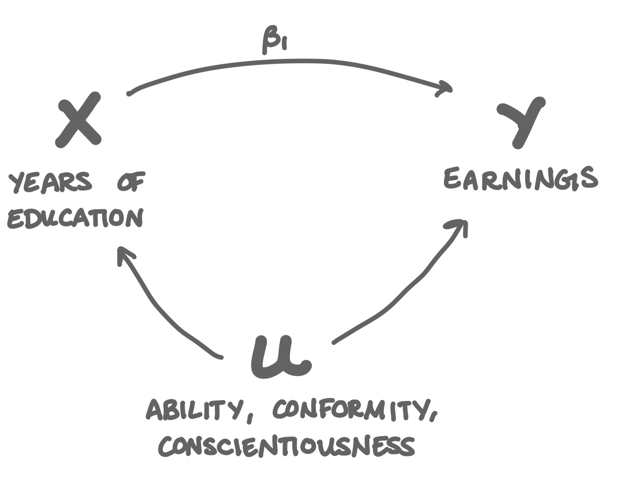
The field of Education Economics is concerned with, more than anything else, this regression:
\[\text{Earnings}_i = \beta_0 + \beta_1 \text{Years of Education}_i + u_i\]
Take any dataset, around the world, throughout history, add as many other explanatory variables as you like (field, industry, gender, experience, parent’s education, etc) and you’ll find that the years someone spends in school seems to have an incredibly large and positive effect on their earnings down the road. And that makes sense: education should give you the skills and the new ways of thinking that ensure you’ll be successful in the real world. If it didn’t, what would be the point?
The thing is, the size of that \(\hat{\beta}_1\) is so large and positive that you have to wonder: if education is such a good investment, why do so many people drop out of high school and college? Why do so many people not go to college (when the cost of student loans is minuscule compared to the boost you seem to get to lifetime earnings)? As economists, we don’t usually like to chalk things up to irrational behavior. There has to be something else going on!
The answer is that there is omitted variable bias in that regression. There are variables that are really important in predicting someone’s earnings, those variables are hard to measure, and those variables are also highly correlated with predicting how much education someone has received. They are: ability, conscientiousness, and conformity (the best discussion of this is certainly Bryan Caplan’s 2018 book The Case Against Education).
High ability people get more education because school is easy for them, and then they go on to have successful careers, but not necessarily because of their educations: they were people with high ability, conscientiousness, and conformity to begin with.
There’s no great way to measure ability, conscientiousness, and conformity, so when we have to leave them out of the earnings ~ education regression, because they’re correlated so strongly with both earnings and education, they confound the earnings-education relationship we’re trying to understand. Given only observational data on people’s salaries and educations, we can never know which one it is.
When we have to omit ability, conscientiousness, or conformity from that earnings-education model, we can’t tell whether someone’s high earnings is because of their education, or because of their high ability, conscientiousness, or conformity. As a result, education always appears to be a much better investment than it actually is.
Simulation
a) Write a helper function that generates a simulated data set.
Complete the following function to generate simulated data where:
- Ability is randomly distributed (hint: use runif for the random uniform distribution)
- Education depends on ability plus random noise
- Earnings depends on both ability and education
- The true effect of ability on earnings should be 2
- The true effect of education on earnings should be 1
b) Demonstrating Bias
Finish the code chunk to run 1000 simulations that:
- Generates data using your function
generate_education_data - Fits a model of
earnings ~ education(omitting ability) - Extracts the education coefficient
- Creates a density plot of the estimates for each of the 1000 simulations
# map(
#   1:1000,
#   function(x) {
#     generate_education_data() %>%
#       lm(_____) %>%
#       broom::tidy() %>%
#       slice(_____) %>%
#       select(_____)
#   }
# ) %>%
#   list_rbind() %>%
#   ggplot(aes(x = _____)) +
#   geom_density() +
#   geom_vline(xintercept = 1)
c) Include the Omitted Variable
Modify your simulation to include ability in the model. You should find that the bias is eliminated.
# map(
#   1:1000,
#   function(x) {
#     generate_education_data() %>%
#       lm(_____) %>%
#       broom::tidy() %>%
#       slice(_____) %>%
#       select(_____)
#   }
# ) %>%
#   list_rbind() %>%
#   ggplot(aes(x = _____)) +
#   geom_density() +
#   geom_vline(xintercept = 1)
Violation of Exogeneity
For OLS to be unbiased, the key assumption is exogeneity: E[u | X] = 0. In this case, that means we have to assume that E[ability | education] = 0. Or in more intuitive terms: two people walk into the room, and you only know their education levels. One person dropped out after the 8th grade, and one person got their PhD. If you had to bet, which person has the higher ability? (Likely the person with their PhD).
If \(X\) gave you no useful information about the value of a person’s \(u\), then exogeneity holds. In this case, exogeneity fails: a person’s education gives you a pretty good idea of what their underlying ability might be. Because exogeneity fails, we can expect OLS to be biased (unless we’re able to add ability or a good proxy for ability to the regression as an explanatory variable).
d) Good News: Prediction is Not Fundamentally at Risk under OVB
While OVB affects causal inference, it may not severely impact prediction. Education acts as a proxy for ability. While the regression overstates education’s importance, we’re still able to do a good job at predicting someone’s earnings. Demonstrate this by:
- Generating training and test data sets
- Fitting a model without ability
- Evaluating prediction accuracy
- Creating a visualization comparing predicted vs actual earnings
train_data <- generate_education_data()
test_data <- generate_education_data()

# test_data %>%
#   mutate(
#     prediction = predict(lm(_____, data = train_data), newdata = test_data),
#     test_error = (earnings - prediction)^2
#   ) %>%
#   summarize(mean_test_error = sqrt(mean(_____)))

# test_data %>%
#   mutate(
#     prediction = predict(lm(_____, data = train_data), newdata = test_data)
#   ) %>%
#   ggplot(aes(x = education, y = earnings)) +
#   geom_point() +
#   geom_line(aes(y = prediction), color = "blue") +
#   labs(title = "Actual vs Predicted Earnings by Education",
#        x = "Years of Education",
#        y = "Earnings")