In the previous assignment, you grew a regression tree to predict the log salaries of major league baseball players based on their performance statistics. While growing a tree, we aim to minimize the Residual Sum of Squares (RSS) by splitting the data into regions. However, a fully grown tree can overfit the training data, leading to poor generalization on unseen data. To address this, we prune the tree by removing branches that contribute little to the model’s predictive power. In this assignment, you will implement weakest link pruning to simplify the tree and improve its performance.
Cost Complexity Pruning
Cost complexity pruning is a technique that involves iteratively removing the least important splits (those that contribute the least to reducing the RSS) from the tree.
The cost complexity measure is defined as:
\(R_{\alpha}(T) = RSS(T) + \alpha \cdot |T|\)
where:
\(RSS(T)\) is the residual sum of squares for the tree T
\(|T|\) is the number of terminal nodes in the tree
\(\alpha\) is a complexity parameter that controls the trade-off between the tree’s complexity and its fit to the data
For weakest link pruning, we choose the subtree that minimizes \(R_{\alpha}(T)\) for a given \(\alpha\).
Here’s a great explanation of the process (we won’t do the cross validation part at the end):
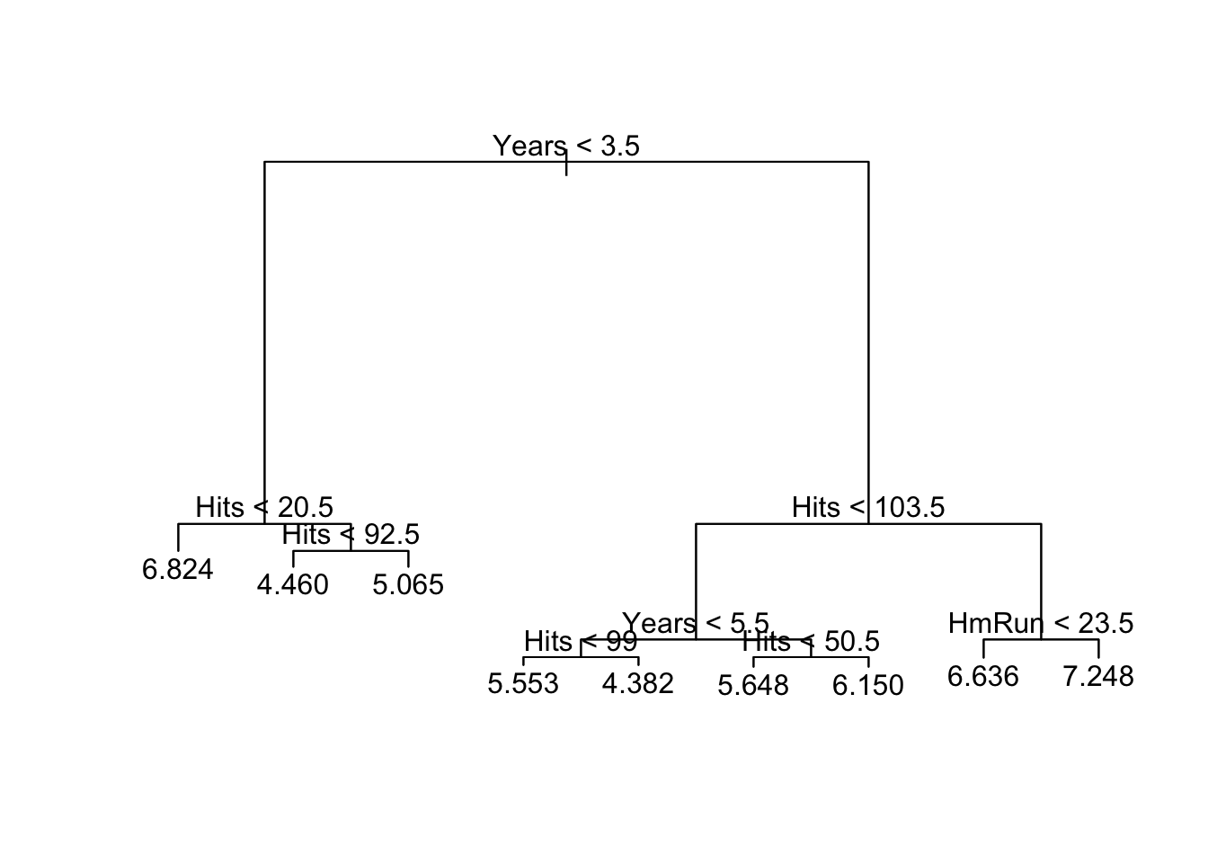
In assignment 5.1, we calculated the RSS for a node as the sum of the RSS from each branch. tree gives the deviance of each branch as the third value when you print model. For example, we found that the first node Years < 3.5 resulted in an RSS of 54.63. tree tells us the deviance of the first branch Years < 3.5 is 8.45, and the deviance of the second branch is Years > 3.5 46.1800. Notice that 8.45 + 46.18 = 54.63, the RSS we found. So here, think of deviance as the same as RSS.
Tree Pruning
RSS for Full Tree
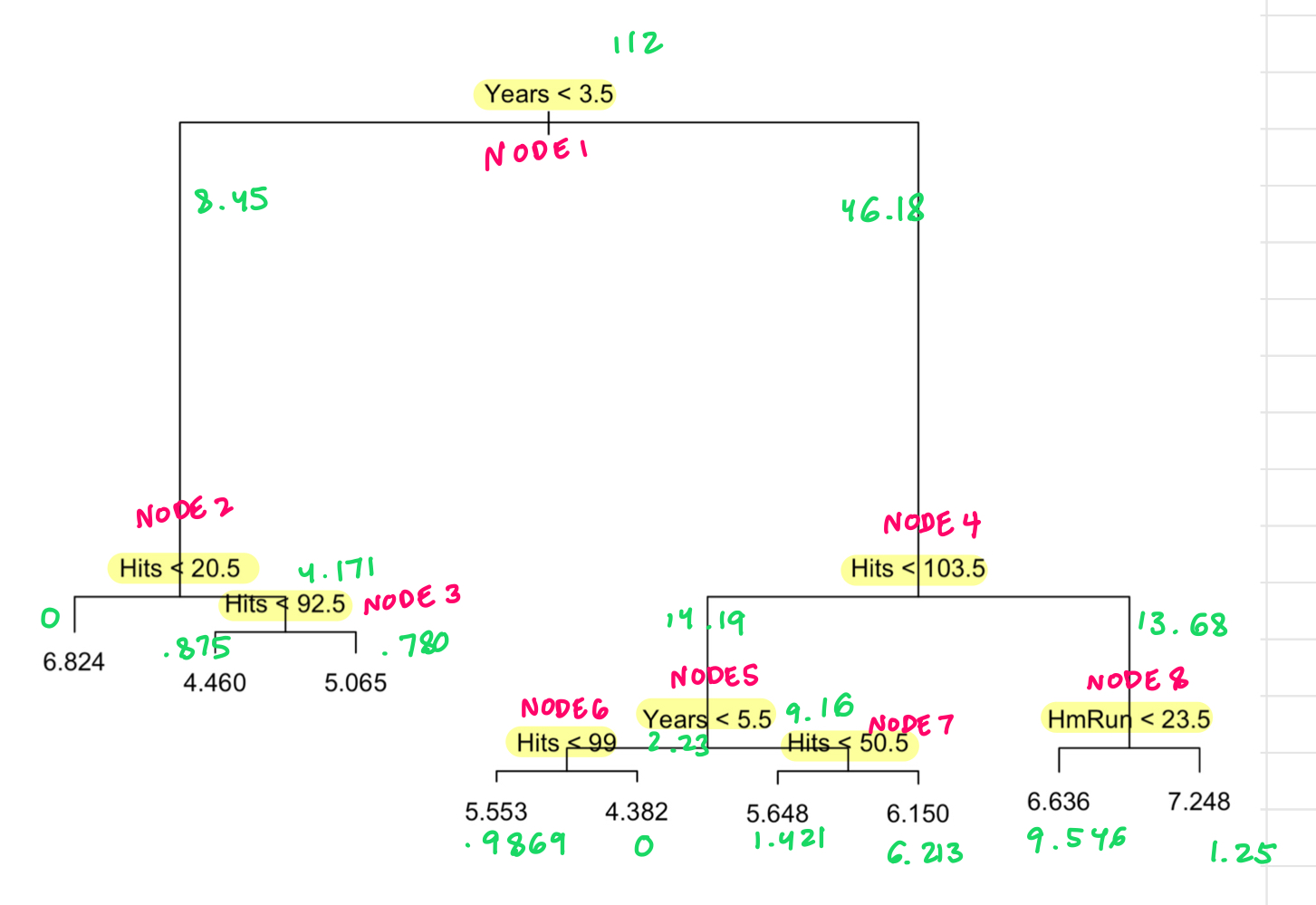
The RSS for the full tree is the deviance of each terminal node:
0+ .875+ .78+ .9869+0+1.421+6.213+9.546+1.25
[1] 21.0719
RSS for Tree Without Node 3
I’ll label nodes like this, and put deviances in green:
If I delete node 3, here’s the RSS for each terminal node now:
0+4.171+ .9869+0+1.421+6.213+9.546+1.25
[1] 23.5879
RSS for the Tree without Node 2
Compute the RSS for the tree, deleting node 2.
Tree Score
Let the tuning parameter be \(\alpha = 3\). Then the Tree Score = RSS + 3 T, where T is the total number of leaves.
Full tree: 21.0719 + 3 * 9 = 48.0719
Without node 3: 23.5879 + 3 * 8 = 47.588
Without node 2: 27.8669 + 3 * 7 = 48.8669
So \(\alpha = 3\) points to eliminating node 3 as the best way to prune on the left hand side of the tree.
Now prune the right hand side of the tree. Compare your answers to how tree prunes the model with k = 3. This results in a much simpler tree without too much loss in predictive power.
Test Error
Compute the test error for the full model (using the test data set instead of training data set).
Compute the test error for the pruned model.
Weakest link pruning is a powerful technique to simplify decision trees and potentially improve their generalization performance. By iteratively removing the least important branches, we can balance model complexity and predictive accuracy. In this assignment, you implemented weakest link pruning and compared the performance of the pruned tree to the fully grown tree. This process is essential for creating interpretable and robust regression trees.