library(tidyverse)
library(ISLR2)
data("USArrests")
arrests <- USArrests %>%
  as_tibble() %>%
mutate(state = rownames(USArrests))6.2 Data Visualization with Principal Component Analysis
Principal components is a tool for dimensionality reduction: it finds the linear combinations of predictors that form directions along which the data varies the most. In assignment 6.1, we saw how principal components can be used in conjunction with linear regression to help with high variance when the number of observations n is small relative to the number of predictors p.
Perhaps an even more useful way to use principal components is for data exploration and visualization. If you have 10 variables and you want to understand the nature of their relationships, you could make scatterplots of each variable with each other variable, but that would mean studying 90 different plots! Instead, use PCA for dimension reduction: reduce the 10 variables down to 2 principal components, then plot the first principal component against the second. In this assignment, we’ll explore how this works.
Question 1: Reviewing 6.1
What is the first principal component?
How is the second principal component different from the first?
How can you calculate principal components?
What benefit does principal component regression have over linear regression?
Question 2
Run this code to load a data set for each state on murder, assault, and rape arrests (per 100,000), and also state’s percent urban population.
- Use
geom_colto visualize which states have the highest to lowest murder rate. (Hint: use fct_reorder() onstateto order the data based on the murder rate). Which 5 states have the lowest murder rate?
# arrests %>%
# ___- Use
geom_colto visualize which states have the highest to lowest assault arrests. Which 5 states have the lowest assault arrests?
# arrests %>%
# ___- Use prcomp() to compute the principal components. Three of the four variables are highly correlated and strongly influence the first principal component. Which three variables are they? The second principal component is influenced primarily by a different variable that is less correlated with the others. Which variable is this?
pca <- prcomp(USArrests, scale = T)
print(pca)
Standard deviations (1, .., p=4):
[1] 1.5748783 0.9948694 0.5971291 0.4164494
Rotation (n x k) = (4 x 4):
PC1 PC2 PC3 PC4
Murder -0.5358995 -0.4181809 0.3412327 0.64922780
Assault -0.5831836 -0.1879856 0.2681484 -0.74340748
UrbanPop -0.2781909 0.8728062 0.3780158 0.13387773
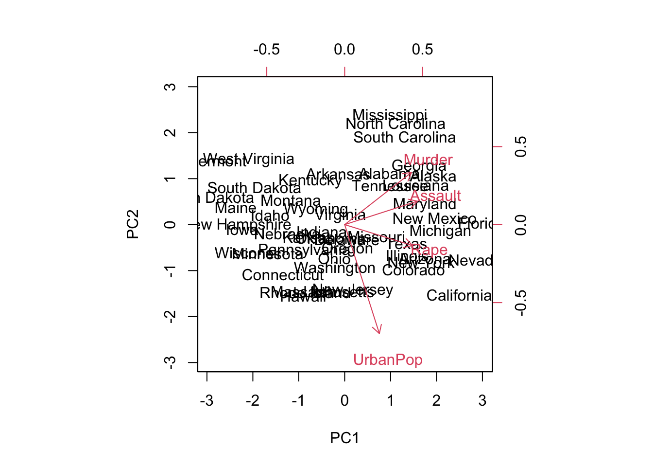
Rape -0.5434321 0.1673186 -0.8177779 0.08902432- Plot the data along with the first two principal components with
biplot(). The first principal component is on the x-axis: it can be interpreted as “crime seriousness” because of your answers in part C. The second principal component is on the y-axis, and it can be interpreted as “urbanization”. Which states have the highest values for both; the lowest values for both; and high values for one but low values for the other?
biplot(pca, scale = 0)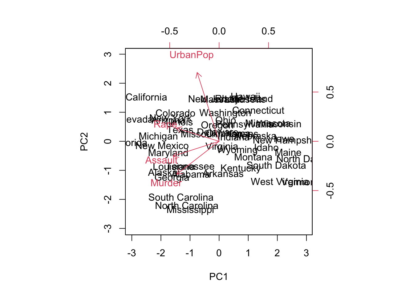
# Flip the direction vectors to indicate "more" to the right:
pca$rotation <- -pca$rotation
pca$x <- -pca$x
biplot(pca, scale = 0)