6.1 Principal Components Regression

Prereq: Constrained Optimization Example

Suppose we wanted to find the maximum of the function \(f(x_1, x_2) = x_1 x_2\), constrained so that \(0 < x_1 < 1\) and \(0 < x_2 < 1\). We should find that the optimum occurs at \(x_1 = 1\) and \(x_2 = 1\), and the optimum is 1.

library(plotly)

# Create a grid of x1 and x2 values
x1 <- seq(0, 1, length.out = 10)
x2 <- seq(0, 1, length.out = 10)

plot_ly(
  x = x1, y = x2, z = outer(x1, x2, "*"),
  type = "surface"
)

Using constrOptim:

Here are the constraints:

\(x_1 > 0\)
\(x_2 > 0\)
\(x_1 < 1\)
\(x_2 < 1\)

Here’s the way we need to transform those constraints to put them into the constrOptim function:

\(x_1 + 0 x_2 > 0\)
\(0 x_1 + x_2 > 0\)
\(-1x_1 + 0 x_2 > -1\)
\(0 x_1 - x_2 > -1\)

constrOptim finds the minimum by default, so if you want to find the maximum, just multiply your function by -1.

constrOptim(
  theta = c(0.1, 0.1), # starting values for the search
  f = function(x) - (x[1] * x[2]), # function to minimize
  ui = matrix(c(1, 0, 0, 1, -1, 0, 0, -1), byrow = T, nrow = 4), # left hand side of the constraints
  ci = c(0, 0, -1, -1), # right hand side of the constraints
  grad = NULL
)

$par
[1] 1 1

$value
[1] -1

$counts
function gradient 
     306       NA 

$convergence
[1] 0

$message
NULL

$outer.iterations
[1] 3

$barrier.value
[1] 1.138706e-10

The results tell us that the maximum happens when \(x_1\) and \(x_2\) are both 1, and the maximum value is 1.

Principal Components Regression

To begin this unit on clustering, we’ll briefly return to the regression model fit with OLS: \(y_i = \beta_0 + \beta_1 x_{1i} + \beta_2 x_{2i} + ... + \beta_p x_{pi} + u_i\). When the number of observations \(n\) is small relative to the number of predictors \(p\), OLS (ordinary least squares) suffers from high variance: different training sets yield very different predictions. An improvement can be made to OLS: principal components regression works to decrease variance at a negligible increase in bias. Principal components regression works through dimension reduction: you’ll project the \(p\) predictors onto an m-dimensional subspace where m < p, and use the m projections as predictors to fit a linear regression with OLS. Principal component analysis is a popular approach for deriving a low-dimensional set of features from a large set of predictors.

The First Principal Component

The first principal component is the direction along which the observations vary the most, defining the line that is closest to the data. For example, if our analysis was only on population and advertising spending, the first principal component is shown in green:

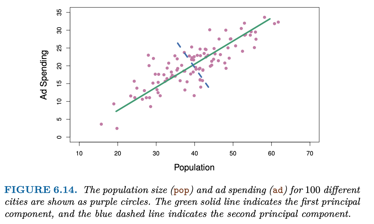
When each data point is projected onto the green line (the principal component), each data point gets assigned a single-number summary \(z\) of the joint population and advertising spending for each location. That is, if z < 0 for an observation, then it likely has a lower than average population and lower than average advertising spending.

Here’s how to construct the first principal component:

Standardize the scale of each predictor by subtracting the mean and dividing by the standard deviation. If you skip this step, then higher variance predictors will play a larger role than lower variance predictors.
Calculate \(z_m\) as the linear combination of predictors: \(z_m = \phi_1 x_1 + \phi_2 x_2 + ... + \phi_P x_P\), where \(\sum_p \phi_p^2 = 1\), and \(\phi_p\) is chosen to find the direction along which the observations vary the most. That is:

\[ \max_{\phi_1, \ldots, \phi_p} \quad \frac{1}{n} \sum_{i = 1}^n \left( \sum_{j = 1}^P \phi_j x_{ij} \right)^2 \quad \mathrm{subject\ to} \quad \sum_{j = 1}^P \phi_{j}^2 = 1 \]

The second principal component is found the same way, but with another constraint: the direction must be perpendicular (orthogonal) to the first principal component. If you keep on constructing principal components, each one must be orthogonal to all previous principal components.

Let’s practice constructing the first principal component for the carseat data from ISLR2:

install.packages("pls")
install.packages("ISLR2")

library(pls)
library(tidyverse)
library(ISLR2)
set.seed(1234)
carseats <- Carseats %>%
  as_tibble() %>%
  select(sales = Sales, ads = Advertising, pop = Population, age = Age, income = Income, education = Education, urban = Urban, price = Price, us = US) %>%
  slice_sample(n = 25) %>%
  mutate(train = c(rep(1, 15), rep(0, 10)))

train <- carseats %>% filter(train == 1) %>% select(-train)
test <- carseats %>% filter(train == 0) %>% select(-train)

Question 1: Use dplyr functions to standardize the variables `ads` and `pop` by subtracting means and dividing by standard deviations.

# train %>%
#   summarize(
#     pop_mean = ___,
#     pop_sd = ___,
#     ads_mean = ___,
#     ads_sd = ___
#   )

# pop_standardized <- train %>%
#   mutate(pop = (pop - ___) / ___) %>%
#   pull(pop)

# ads_standardized <- train %>%
#   mutate(ads = (ads - ___) / ___) %>%
#   pull(ads)

Question 2: Use constrained maximization to calculate \(\phi_1\) and \(\phi_2\) to form the first principal component: a linear combination of `pop` and `ads` along the direction where the data varies the most.

We need to use nloptr instead of constrOptim because our constraints is the nonlinear constraint \(\phi_1^2 + \phi_2^2 = 1\). The number of predictors p is equal to 2 (pop and ads). You’ll use pop_standardized and ads_standardized, and your theta is \(\phi_1\) and \(\phi_2\).

library(nloptr)

# objective function
f <- function(x) {
  # value <- (-1 / 15) * sum(___)
  
  grad <- c(
    (-2 / 15) * sum((pop_standardized * x[1] + ads_standardized * x[2]) * pop_standardized),
    (-2 / 15) * sum((pop_standardized * x[1] + ads_standardized * x[2]) * ads_standardized)
  )
  
  return(list("objective" = value, "gradient" = grad))
}

# Nonlinear constraint
sum_squares_1 <- function(x) {
  return(list("constraints" = x[1]^2 + x[2]^2 - 1,
              "jacobian"    = c(2*x[1], 2*x[2])))
}

nloptr(
  x0 = c(1, 0), # starting values for the search
  eval_f = f, # function to minimize
  eval_g_eq = sum_squares_1,
  opts = list("algorithm" = "NLOPT_LD_SLSQP", "xtol_rel" = 1e-8)
)

# Visualizing the first principal component against the data
tibble(
  pop = pop_standardized,
  ads = ads_standardized
) %>%
  ggplot(aes(x = pop, y = ads)) +
  geom_point() +
  stat_function(fun = function(x) x)

# Principal Component Regression
lm(sales ~ I(.706 * pop_standardized + .708 * ads_standardized), data = train)

Question 3: Find the training MSE for this PCR.

# train %>%
#   mutate(prediction = ___) %>%
#   summarize(mse = mean(___))

Compare this to the pcr.fit results.

pcr.fit <- pcr(sales ~ pop + ads, data = train, scale = T, ncomp = 1)

Question 4: Find the training MSE with the PCR from the `pcr` function.

# train %>%
#   mutate(prediction = predict(pcr.fit, data = .)) %>%
#   summarize(mse = mean(___))

Principal Component Regression for all Predictors

pcr.fit <- pcr(sales ~ ., data = train, scale = T, ncomp = 5)
summary(pcr.fit)

summary() provides the percentage of variance explained in the predictors and in the response using different numbers of components. Using M = 1 captures 30% of all the variance in the predictors. Using M = 5 increases the value to 92.34%.

Perform PCR on the training data and evaluating its test performance:

test %>%
  mutate(prediction = predict(pcr.fit, test, ncomp = 5)) %>%
  summarize(mse = mean((sales - prediction)^2))

Compare this to least squares MSE:

ls_fit <- lm(sales ~ ., data = train)
test %>%
  mutate(prediction = predict(ls_fit, test)) %>%
  summarize(mse = mean((sales - prediction)^2))