library(tidyverse)
hitters <- read_csv("https://raw.githubusercontent.com/cobriant/teaching-datasets/refs/heads/main/hitters.csv") %>%
  mutate(Salary = log(Salary))

train <- hitters %>%
  filter(training == 1) %>%
select(-training)5.1 Growing a Regression Tree
A decision tree is a method that can be used for regression problems (the dependent variable is continuous), or classification problems (the dependent variable is discrete). In this assignment, you’ll practice growing a regression decision tree to estimate 1987 salaries of major league baseball players based on their hits, runs, and home runs the previous season (1986), along with the number of years they had spent in the major leagues.
Like K Nearest Neighbors, decision trees do well at estimating highly nonlinear, complex relationships between variables. But compared to KNN, decision trees are much easier to interpret: in fact, they are even easier to interpret than linear regression! Here’s an example of a simple decision tree on baseball player salaries in logs:
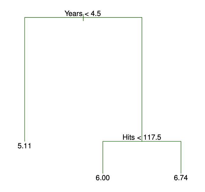
This tree has two internal nodes and three terminal nodes. The left-hand branches correspond to “TRUE” and the right-hand branches correspond to “FALSE”. So players with less than 4.5 years of experience have a predicted log salary of 5.11. For more experienced players, the number of hits they had in the previous season is found to be highly predictive of salary.
Decision trees segment the predictor space into rectangular regions, and the prediction is the average salary in the training set for that region. At each branch, you’ll consider all predictors and all cutpoints \(s\), selecting the predictor and cutpoint that minimizes the RSS (residual sum of squares). Continue until all regions have a sufficiently small number of training observations.
In this assignment, we’ll work on growing a decision tree by hand. Then we’ll compare our decision tree to the one created with the R package tree.
dense_rank
The dplyr function dense_rank gives a rank to each value in a vector, and ties get the smaller value. For example:
df <- tibble(x = c(5, 3, 3, 3, 8, 4))

df %>%
  mutate(r = dense_rank(x))
# A tibble: 6 × 2
x r
<dbl> <int>
1 5 3
2 3 1
3 3 1
4 3 1
5 8 4
6 4 2This will be really helpful in this assignment. In particular, we’ll use it to create regions with smaller values versus larger values, preserving ties in the same region. If we want to create a region with the first rank versus another region with all other ranks:
n <- 2

df %>%
  mutate(region = if_else(dense_rank(x) < n, "small", "large"))
# A tibble: 6 × 2
x region
<dbl> <chr>
1 5 large
2 3 small
3 3 small
4 3 small
5 8 large
6 4 large - Consider
HmRunand the training data settrain. This variable takes on 35 distinct values in this data set (between 0 and 40 home runs in the previous season). If you create two regions using a cutpoint of the 5th value for HmRun (H >= H5 or H < H5), and you predict the average salary for each region, what is the RSS and predicted log salaries for players above and below that cutpoint?
hitters %>% count(HmRun)# A tibble: 35 × 2
HmRun n
<dbl> <int>
1 0 10
2 1 10
3 2 12
4 3 14
5 4 17
6 5 18
7 6 14
8 7 13
9 8 16
10 9 12
# ℹ 25 more rows# train %>%
# select(Salary, HmRun) %>%
# mutate(
# rank = ___,
# region = if_else(rank >= 5, "high", "low")
# ) %>%
# group_by(___) %>%
# summarize(
# prediction = mean(___),
# RSS = sum((___)^2),
# variable_min = min(HmRun)
# ) %>%
# reframe(RSS = sum(RSS), region, prediction, cutpoint = max(variable_min)) %>%
# pivot_wider(names_from = region, values_from = prediction)Interpretation: players with less than ___ home runs last season receive a log salary of ___ on average; players with ___ or more home runs last season receive a log salary of ___ on average. Cutting home runs at this point gives an RSS of ___.
RSS Helper Function
- Repeat the process from question 1, this time writing a helper function
RSSthat takes a variable and a cutpoint rank number, and returns the RSS and the cutpoint.
# RSS <- function(variable, cut_rank, dataset) {
#   dataset %>%
#     select(Salary, {{ variable }}) %>%
#     ___
# }

# Test: you should get the same answer as in question 1
# RSS(HmRun, 10, train)
Cutpoint Helper Function
- Write another helper function
cutpointthat takes a variable and searches over all possible cut rank numbers to find the cutpoint that results in the lowest possible RSS. Your function should return the RSS, the best cutpoint, and the predicted salary for players below and above that cutpoint. Make sure to useRSSalong withmap.
# cutpoint <- function(variable, dataset) {
#   max_rank <- dataset %>%
#     distinct({{ variable }}) %>%
#     nrow()
#
#   map(
#     .x = 1:max_rank,
#     .f = function(x) {
#       ___
#     }
#   ) %>%
#     list_rbind() %>%
#     slice_min(___)
# }

# cutpoint(HmRun, train)
Interpretation: the best cutpoint for home runs are ___ home runs. Players with less than ___ home runs last season receive a salary of ___ on average; players with ___ or more home runs last season receive a salary of ___ home runs on average. Cutting home runs at this point gives an RSS of ___.
Variable Search Helper Function
- Write another helper function
variable_searchthat searches over all explanatory variables and cutpoints to find the explanatory variable and cutpoint that minimizes the RSS.
# variable_search <- function(dataset) {
#   vars <- dataset %>% select(-Salary) %>% names()
#   map(
#     ___,
#     function(varname) {
#       var_sym <- sym(varname)
#       cutpoint(!!var_sym, dataset) %>%
#         mutate(var = varname)
#     }
#   ) %>%
#     list_rbind() %>%
#     slice_min(___, n = 1)
# }

# variable_search(train)
Interpretation: the first node in the tree will be ___ < . For players with , the average log salary is , and for players with , the average log salary is . This cutpoint yields an RSS of .
Grow the Tree
- Drill into each region from
variable_search(train), growing a subtree. Stop growing a branch after it reaches a depth of 4 nodes. It will probably be useful to draw the tree on a sheet of paper as you’re working.
Compare your tree: tree package
install.packages("tree")library(tree)
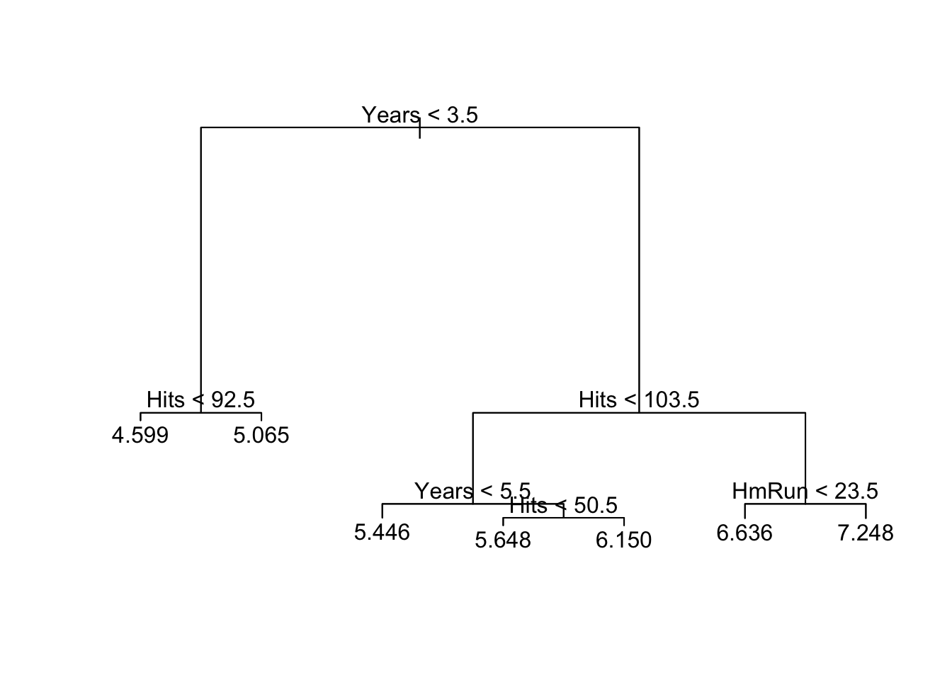
bb_tree <- tree(Salary ~ Hits + Years + Runs + HmRun, data = train)
bb_treenode), split, n, deviance, yval
* denotes terminal node
1) root 136 112.0000 6.040
2) Years < 3.5 29 8.4500 4.792
4) Hits < 92.5 17 6.1380 4.599 *
5) Hits > 92.5 12 0.7804 5.065 *
3) Years > 3.5 107 46.1800 6.378
6) Hits < 103.5 44 14.1900 5.883
12) Years < 5.5 11 2.2330 5.446 *
13) Years > 5.5 33 9.1610 6.028
26) Hits < 50.5 8 1.4210 5.648 *
27) Hits > 50.5 25 6.2130 6.150 *
7) Hits > 103.5 63 13.6800 6.724
14) HmRun < 23.5 54 9.5460 6.636 *
15) HmRun > 23.5 9 1.2500 7.248 *bb_tree %>% summary()
Regression tree:
tree(formula = Salary ~ Hits + Years + Runs + HmRun, data = train)
Variables actually used in tree construction:
[1] "Years" "Hits"  "HmRun"
Number of terminal nodes:  7
Residual mean deviance:  0.2138 = 27.58 / 129
Distribution of residuals:
     Min.   1st Qu.    Median      Mean   3rd Qu.      Max.
-1.545000 -0.318800 0.006428 0.000000 0.260900 2.226000 plot(bb_tree)
text(bb_tree)