move <- function(cell, action) {
  if (action == ___) {
    return(cell)
  } else if (action == ___) {
    if (cell <= 6) {
      return(cell + 3)
    } else {
      return(cell)
    }
  } else if (action == ___) {
    ___
  } else if (action == ___) {
    ___
  } else if (action == ___) {
    ___
  }
}4.2 Dynamics Part 1
Payoff Function
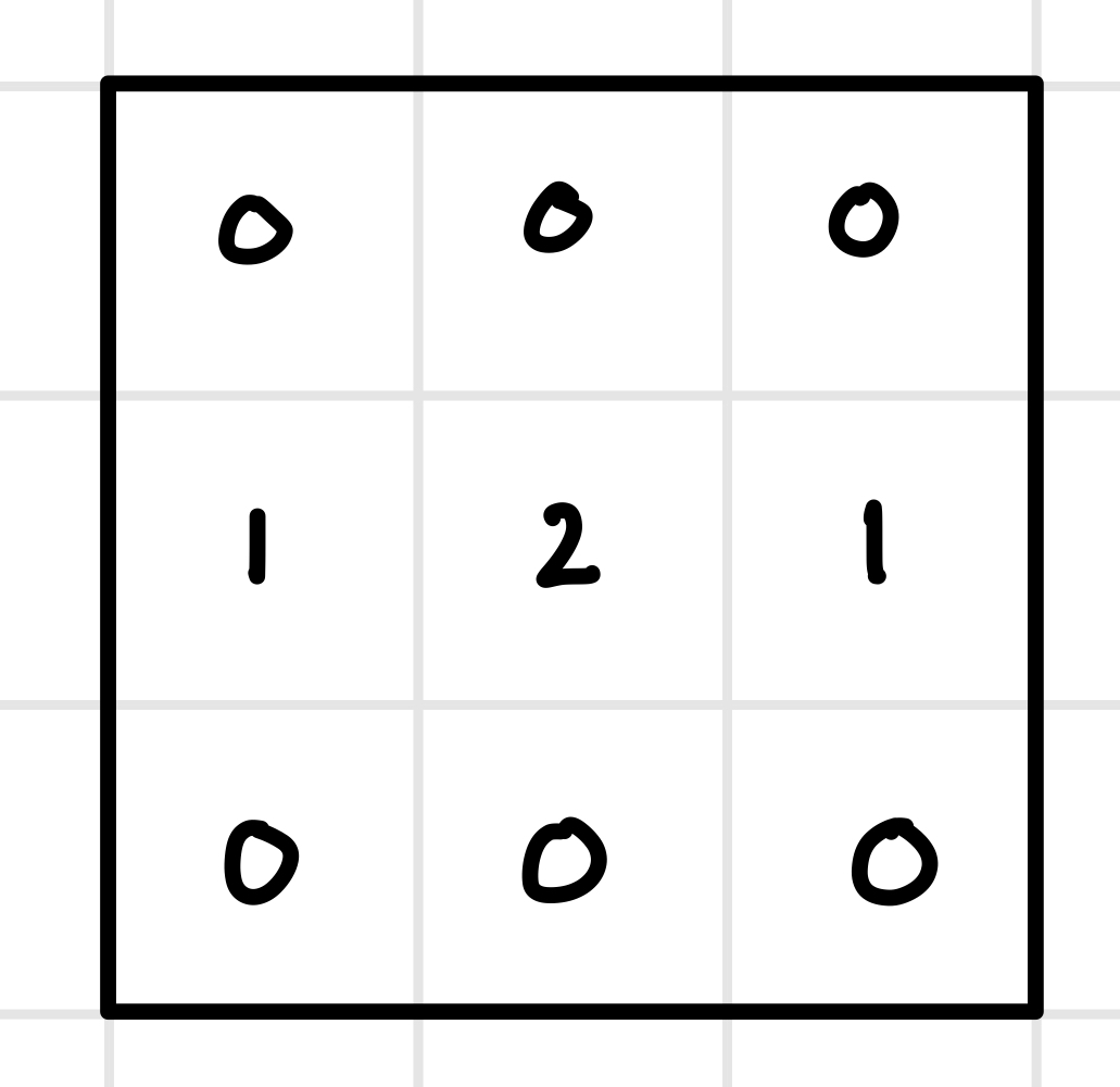
Consider a game where an agent has a random initial starting position on one cell of a 3x3 “GridWorld”. The agent takes sequential actions (north, south, east, west, or stay), and their objective is to maximize the sum of their payoffs. The payoffs for each cell are labeled: cells in the first and third rows have a payoff of zero each, and cells in the second row have payoffs 1, 2, and 1. If the agent takes an action toward the boundary, they stay in the same cell as before.
Policy Function
- Write down the policy function for the agent: a set of best responses given they are in each cell. For instance, if they find themselves in cell 1 (upper left), they should choose to go south because that will help them maximize the sum of their payoffs.
| position | best responses |
|---|---|
| 1 (upper left) | south |
| 2 (upper middle) | ___ |
| 3 (upper right) | ___ |
| 4 (center left) | ___ |
| 5 (center) | ___ |
| 6 (center right) | ___ |
| 7 (lower left) | ___ |
| 8 (lower middle) | ___ |
| 9 (lower right) | ___ |
Value Function (AKA Bellman Equation)
The value function represents the value of being in a particular cell, defined as the sum of future payoffs assuming the agent follows the policy function (their optimal strategy). For example, consider the value of being in cell 5, the center of the grid. If the agent remains in the center, the value is calculated as \(V_5 = 2 + 2 + 2 + 2 + \dots\). However, this value does not converge: it grows infinitely, which poses a problem when comparing the value of one cell to another (since every cell’s value would also be infinite). To address this, we adjust the definition of the value function to be the discounted sum of future payoffs, assuming the agent follows the policy function. Introducing a discount rate of 0.9, the value function now accounts for the fact that future payoffs are worth less than immediate ones. This ensures that the value of each cell converges to a finite number, allowing for meaningful comparisons between cells. For instance, the revised value of being in cell 5 would be calculated as \(V_5 = 2 + .9 \cdot 2 + .9^2 \cdot 2 + .9^3 \cdot 2 + \dots\), which converges to a finite value. This adjustment makes the value function a practical tool for decision-making and analysis.
Another interpretation for the discount rate is that the game could end at each time step with probability 0.1 (or, equivalently, continue with probability 0.9). In this case, the discount rate reflects the likelihood that the game will continue into the future. Under this interpretation, the value function represents the expected value of being in each state, taking into account the possibility that the game might terminate at any point. For example, if the agent is in cell 5, the value \(V_5\) is not just the sum of future payoffs but the expected sum, weighted by the probability that the game continues at each step. This probabilistic framing aligns with the discounted sum approach, as both account for the diminishing importance of payoffs further in the future.
Steps for solving a discounted sum of payoffs: \(V_5 = 2 + .9 \cdot 2 + .9^2 \cdot 2 + .9^3 \cdot 2 + \dots\)
- Notice that subtracting 2 from \(V_5\) yields the same thing as multiplying \(V_5\) by 0.9: \(V_5 - 2 = .9 V_5\)
- Take that equation and solve for \(V_5\): \(.1 V_5 = 2\), so \(V_5 = 20\).
- Solve for the value of being in each cell on the grid. Start with \(V_4\) and \(V_6\): notice they are \(1 + .9 V_5\).
| position | value |
|---|---|
| 1 | ___ |
| 2 | ___ |
| 3 | ___ |
| 4 | ___ |
| 5 | \(V = 2 + .9(2) + .9^2(2) + .9^3(2) + \dots = 20\) |
| 6 | ___ |
| 7 | ___ |
| 8 | ___ |
| 9 | ___ |
Note that if the agent knows the value function, they can derive the policy function by taking the action that moves them toward the cell with the highest value.
- Consider an agent who starts in cell 1. They could stay (\(V_1 = 17.1\)), move east (\(V_2 = 18\)), or move south (\(V_4 = 19\)). They move south because that has the highest value.
Programming Solution
- Write a helper function to define movement on the grid.
- Test your function
moveusing the functiontest_thatfrom R packagetestthat.
library(testthat)

test_that("move function works correctly", {
  # Test "stay" action
  expect_equal(move(5, "stay"), 5)

  # Test "south" action
  expect_equal(move(2, "south"), ___)  # Valid move
  expect_equal(move(7, "south"), ___)  # Invalid move (out of bounds)

  # Test "north" action
  expect_equal(move(8, "north"), ___)  # Valid move
  expect_equal(move(2, "north"), ___)  # Invalid move (out of bounds)

  # Test "east" action
  expect_equal(move(1, "east"), ___)   # Valid move
  expect_equal(move(3, "east"), ___)   # Invalid move (out of bounds)

  # Test "west" action
  expect_equal(move(2, "west"), ___)   # Valid move
  expect_equal(move(1, "west"), ___)   # Invalid move (out of bounds)
})
Write a function
value_iterationthat takes:- a vector of payoffs of length 9
- a
movefunction that defines movement on the grid - a discount rate (default is 0.9)
- a threshold for convergence (default is 0.0001)
Your function should work like this:
- Create two vectors of length 9:
valueandvalue_updateso we can evaluate when we get convergence. They must not be equal. - Begin a while loop that keeps going as long as value and value_update have not converged: that is, as long as the maximum of the absolute value of the difference between value and value_update is larger than the threshold.
- The first thing in the while loop should be to set
value <- value_update. I’m thinking of value as holding the old numbers, and value_update as holding the new numbers. - Write a for loop inside the while loop that iterates over each cell in the grid (1-9). Create variables like
value_stayandvalue_north, which are the value of the cell you get to when you stay or when you go north:value[move(cell, "stay")]orvalue[move(cell, "north")]. Thenvalue_maxshould be the maximum out of those values. - The final step in the for loop is to set value_update[cell] to be the payoff for the cell plus the discount rate times value_max.
- Finally, return
round(value_update, digits = 2).
value_iteration <- function(payoffs, move, discount = 0.9, threshold = 0.0001) {

  value <- ___
  value_update <- ___

  # Continue until value and value_update converge
  while (___) {
    # Store the current values for comparison
    value <- value_update

    # Update the value for each cell
    for (___) {
      # Calculate the value for each action
      value_stay <- ___
      value_north <- ___
      value_south <- ___
      value_east <- ___
      value_west <- ___
      value_max <- ___
      value_update[cell] <- ___
    }
  }
  return(___)
}

# Test your function
value_iteration(c(0, 0, 0, 1, 2, 1, 0, 0, 0), move)
Your answers should match the ones we derived analytically in part B.
- Now use
value_iterationto find the value function for a new GridWorld:
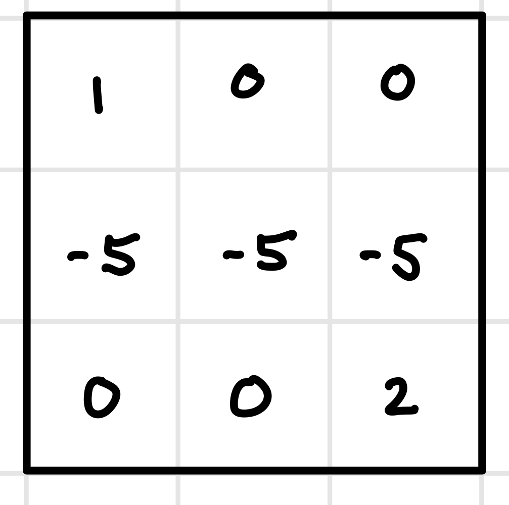
value_iteration(c(___), move) %>% matrix(nrow = 3, byrow = T)- Use the results from part F to write down the policy function for an agent making sequential choices around this GriwdWorld.
| position | action |
|---|---|
| 1 | ___ |
| 2 | ___ |
| 3 | ___ |
| 4 | ___ |
| 5 | ___ |
| 6 | ___ |
| 7 | ___ |
| 8 | ___ |
| 9 | ___ |
- Play with different discount rates in this new GridWorld: how low does the discount rate need to go for an agent starting at position 1 to want to stay there instead of moving toward position 9?