# the tidyverse
install.packages("tidyverse", dependencies = TRUE)
library(tidyverse)

# gapminder
install.packages("gapminder")
library(gapminder)

# install some packages for special plots
install.packages("gganimate", dependencies = TRUE)
install.packages("hexbin")

# another package I developed called qelp (quick help) for beginner-friendly help docs
install.packages("Rcpp", dependencies = TRUE)
install.packages("devtools", dependencies = TRUE)
library(devtools)
install_github("cobriant/qelp")

# Run this:
?qelp::install.packages

# If everything went right, the help docs I wrote on the function `install.packages`
# should pop up in the lower right hand pane.1.1 Vectors, Tibbles, and Pipes
Introduction
Here is my favorite introduction to a programming book, taken directly from Structure and Interpretation of Computer Programs by Gerald Jay Sussman, Hal Abelson, and Julie Sussman:
We are about to study the idea of a computational process. Computational processes are abstract beings that inhabit computers. As they evolve, processes manipulate other abstract things called data.
The evolution of a process is directed by a pattern of rules called a program. People create programs to direct processes. In effect, we conjure the spirits of the computer with our spells.
A computational process is indeed much like a sorcerer’s idea of a spirit. It cannot be seen or touched. It is not composed of matter at all. However, it is very real. It can perform intellectual work. It can answer questions. It can affect the world by disbursing money at a bank or by controlling a robot arm in a factory. The programs we use to conjure processes are like a sorcerer’s spells. They are carefully composed from symbolic expressions in arcane and esoteric programming languages that prescribe the tasks we want our processes to perform.
A computational process, in a correctly working computer, executes programs precisely and accurately. Thus, like the sorcerer’s apprentice, novice programmers must learn to understand and to anticipate the consequences of their conjuring. Even small errors (usually called bugs or glitches) in programs can have complex and unanticipated consequences.
Fortunately, learning to program is considerably less dangerous than learning sorcery, because the spirits we deal with are conveniently contained in a secure way. Real-world programming, however, requires care, expertise, and wisdom. A small bug in a computer-aided design program, for example, can lead to the catastrophic collapse of an airplane or a dam or the self-destruction of an industrial robot.
Master software engineers have the ability to organize programs so that they can be reasonably sure that the resulting processes will perform the tasks intended. They can visualize the behavior of their systems in advance. They know how to structure programs so that unanticipated problems do not lead to catastrophic consequences, and when problems do arise, they can debug their programs. Well-designed computational systems, like well-designed automobiles or nuclear reactors, are designed in a modular manner, so that the parts can be constructed, replaced, and debugged separately.
R’s Benefits
There are countless programming languages we could learn, so why choose R—particularly the tidyverse ecosystem? Here’s why:
1. Beginner-Friendly Syntax
R’s syntax, especially when using the tidyverse, is intuitive and approachable for beginners. If you start with the right approach, you can quickly transition from having no programming experience to tackling complex data problems. R allows you to focus on the bigger picture (determining what you want to compute, breaking problems into manageable parts, and solving them) without getting bogged down by overcomplicated syntax.
2. Industry-Leading Data Visualization with ggplot2
ggplot2, the tidyverse’s visualization package, is a game-changer in data science. It set the gold standard for data visualization, and tools in other programming languages often aim to replicate its capabilities. Mastering ggplot2 is not only essential for creating compelling visualizations but is also a highly marketable skill in the data industry.
3. Transferable Programming Skills
While each programming language has unique features, the core principles of programming are universal. Just like the advice “The best diet is the one you can stick to,” the best programming language is the one you can master and feel comfortable using. Once you become proficient in R, learning other programming languages becomes exponentially easier, as you’ll have a strong foundation in problem-solving and computational thinking.
In short, R and the tidyverse offer a powerful, beginner-friendly, and industry-relevant toolkit to jumpstart your journey into programming and data science. Not to mention, using the tidyverse is just great fun. I hope you’ll agree: it’s easy to use R to create simple, elegant solutions to all kinds of complicated data analytics problems, which is a wonderful thing.
R’s Shortcomings
R is a highly capable engine for data analytics, but you might occasionally hear criticisms like “R is slow.” So, what’s the truth? Is it a good language or not?
Here’s my perspective: before writing a program, you generally have a vague idea of how you want to solve a problem. Writing the program forces you to break down and formalize each step, clarifying your ideas along the way. By the time you’ve finished, you often understand the problem on a much deeper level. This is the intellectual value of programming, and R excels at this task. In fact, thanks to the tidyverse’s emphasis on functional and declarative programming, R often makes it easier to think abstractly, work at a high level, and manipulate large datasets efficiently rather than handling data point by point.
That said, R can face scalability issues. For most typical use cases, R works well, especially with datasets of up to a few million rows. However, for significantly larger datasets, like those with billions of rows, you might notice R slowing down or even crashing. In such cases, you can often break the task into smaller chunks and continue using R. Alternatively, you might need to re-implement your solution in a language like Rust, Java, or C. For truly massive datasets, like trillions of rows, distributed computing frameworks like Spark or Flink allow you to spread the workload across multiple computers.
In summary, R is an excellent choice for developing your initial solution, helping you think through and solve the problem at hand. If performance becomes an issue for larger-scale problems, you can always translate your solution into the most suitable technology for the job.
What Makes Code “Good”?
Let’s define the goals of writing good code:
Good code produces the correct answer.
This is the baseline requirement: if your code doesn’t run, produces errors, or fails to compile, it’s not ready to submit. Keep refining it, collaborate with your groupmates, and seek help during office hours if needed. However, once your code gives the correct result, you’ve reached a functional stopping point.
Good code solves the problem in the simplest way possible.
Simplicity is key. Learn to use tidyverse functions appropriately and avoid mixing tidyverse and base R unnecessarily, as they are separate ecosystems. Overly complex solutions, especially those blending these systems, are common online and are a telltale sign that ChatGPT was involved. (Yes, ChatGPT often makes this mistake.) If you’re unsure how to use a tidyverse function, consult the documentation to improve your understanding and skill.
Good code is clear and readable to others.
As Harold Abelson states in Structure and Interpretation of Computer Programs: “Programs must be written for people to read, and only incidentally for machines to execute.” Clear and readable code aligns with simplicity—when your solution is simple, it’s easier for others (and your future self) to understand.
Good code includes meaningful comments.
Comments should explain why you’re doing something, not just what the code does. A common mistake, also often made by ChatGPT, is to provide surface-level comments that restate the code’s function. Instead, write comments that add value by explaining the reasoning behind your approach. Assume your audience understands the tidyverse and focus on providing insight. These thoughtful comments will also help you when you revisit your code later, providing clarity on decisions you might otherwise forget.
Setting up your workspace
Grab a Computer
First things first, you should decide which computer you’d like to do your programming assignments on. It can be a Mac, Windows, or Linux machine: all are equally good. I do absolutely everything on my little macbook air laptop. Please let me know ASAP if you don’t have a computer to program on (chromebooks and ipads won’t work but there are workarounds I can discuss with you).
Install R and RStudio
Go here: https://cran.r-project.org/ and follow the instructions to download R for your Linux, Windows, or Mac. You should download the latest release.
Then go here: https://posit.co/download/rstudio-desktop/ and click the blue button that says step 2: install RStudio Desktop.
Mac users: make sure you know whether you have an Apple silicon mac or an older intel-based mac and make sure that you download the correct version of R. If you’re using a mac, you’ll also need to install xquartz: https://www.xquartz.org/.
Install a few more packages
Open RStudio and find your “console” pane. Execute these lines of code in your console:
Download the koans
Go here: https://github.com/cobriant/tidyverse_koans and hit the green button that says Code and then hit Download Zip.
Find the file (probably in your downloads folder). On Macs, opening the file will unzip it. On Windows, you’ll right-click and hit “extract”. Then navigate to the new folder named tidyverse_koans and double click on the R project tidyverse_koans.Rproj. RStudio should open. If it doesn’t, open RStudio and go to File > Open Project and then find tidyverse_koans.Rproj.
In RStudio, go to the lower righthand panel and hit the folder R. This takes you to a list of exercises (koans, pronounced “cones”).
Open the first koan: K01_vector.R. Before you start, modify a keybinding:
Macs: Tools > Modify keyboard shortcuts > Run a test file > Cmd Shift T
Windows: Tools > Modify keyboard shortcuts > Run a test file > Ctrl Shift T
Now hit Cmd/Ctrl Shift T. You’ve just tested the first koan. You should see:
[ FAIL 0 | WARN 0 | SKIP 10 | PASS 0 ]
What does this mean? If there are errors in your R script, the test will not complete. Since it completed, you know there are no errors. Since FAIL is 0, you also haven’t failed any of the questions yet. But PASS is also 0, so you haven’t passed the questions either. Since they’re blank right now, the test will skip them. That’s why SKIP is 10.
Go ahead and start working on the koans and learning about the tidyverse! When you’re finished with a koan and the tests pass, it can be nice to be able to see your work in a compiled html document (Ctrl/Cmd Shift K or File > Compile Report).
One last thing: whenever you want to work on the koans, make sure you open RStudio by opening the “tidyverse_koans-master” project, not just the individual koan file. If you open the koans in a session that’s not associated with the “tidyverse_koans-master” project, the tests will fail to run. You can always see which project your current session is being associated with by looking at the upper right hand corner of RStudio: if you’re in the “tidyverse_koans-master” project, you’ll see “tidyverse_koans-master” up there. That’s good. If you’re in no project at all, you’ll see “Project: (None)” up there. That’s not good, especially if you want the tests to run. If you see “Project: (None)”, just click that text and you’ll be able to switch over to the “tidyverse_koans-master” project.
Vectors
In R, data is held in vectors. You can construct a vector using the function c(), which is short for “combine”. That is, in R, you combine elements to form a vector.
- For example, you combine numbers to form a numeric vector:
c(5, 3, 9)[1] 5 3 9- You can combine character strings to form a character vector:
c("apple", "banana", "strawberry")[1] "apple" "banana" "strawberry"Note that character strings like “apple” must be enclosed in quotes, while numbers and functions like c() must not be wrapped in quotes. Here’s why:
- The symbol
3refers to the number 1 + 1 + 1. - The symbol
c()refers to a function that creates a vector. - However, the character string “apple” doesn’t represent or refer to anything—it’s just the sequence of characters a-p-p-l-e grouped together.
If you’re unsure whether something should have quotes, ask yourself: Does it refer to something? If it does, don’t use quotes. If it doesn’t, quotes are required.
You’re now ready to do koan 1 on vectors. As you’re working on it, make sure to run the tests so you can check your answers.
In koan 1, you’ll learn:
- math operators work on vectors:
+ - / * ^ - other functions like
min()andsum()work on vectors length()finds the number of elements in a vector- you can create a vector where elements are repeated using the function
rep() - you can create a vector that does random sampling from another vector using the function
sample()
To turn in this part of the assignment, include koan 1 in its entirety with your answers filled in with the rest of your work for this unit.
Tibbles
Tibbles are tidyverse spreadsheets. Data is still being held in vectors (column vectors specifically), but the rows of the tibble also hold meaning. The rows are the observations while the columns are the variables. This is tricky to understand, so let’s do an example:
Consider the daily weather. Let’s write down each day’s high temperature, low temperature, and rainfall. In words, here’s our data:
- On Jan 1, 2023 we had a high of 46 degrees, a low of 37 degrees, and 0.07 inches of rain.
- On Jan 2, 2023 we had a high of 46 degrees, a low of 35 degrees, and 0.00 inches of rain.
- On Jan 3, 2023 we had a high of 47 degrees, a low of 34 degrees, and 0.08 inches of rain.
Since rows are observations, each day will be a row.
Since variables are columns, we’ll have four columns representing each thing we measured: the date, the high temperature, the low temperature, and the rainfall.
So we want the tibble to look like this:
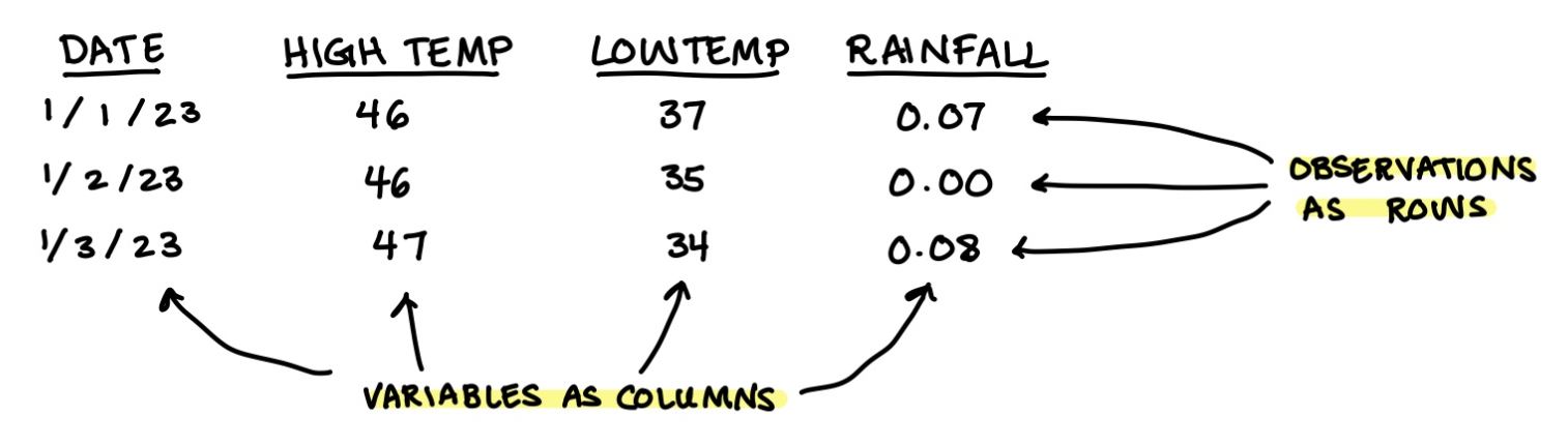 The mantra “observations as rows; variables as columns” is what is called the “tidied data format”. There are tons of ways you could format your data, but the tidyverse is compatible with only this way. Luckily, it turns out to be a very expressible way to format data.
Here’s the code to construct a tibble:
# The function tibble() comes from the tidyverse, so make sure you have the tidyverse attached in your current R session
library(tidyverse)

# tibble() takes a comma separated list of named columns, and returns a tibble, which is a type of data frame.
tibble(
  date = as.Date(c("2023-01-01", "2023-01-02", "2023-01-03")),
  high_temp = c(46, 46, 47),
  low_temp = c(37, 35, 34),
  rainfall = c(0.07, 0, 0.08)
)
# A tibble: 3 × 4
date high_temp low_temp rainfall
<date> <dbl> <dbl> <dbl>
1 2023-01-01 46 37 0.07
2 2023-01-02 46 35 0
3 2023-01-03 47 34 0.08Tibbles have 2 rules:
Each column must be named. Here, the column (variable) names are date, high_temp, low_temp, and rainfall. If you try to define a column without giving it a name,
tibble()will generate one for you. It usually isn’t pretty. You can try this: take the code above and delete thedate =.Each column must have the same number of rows. If you try to define one column that’s shorter than the others,
tibble()will give you an error. (Exception: if you define a column with only one element, tibble will repeat that one element to make it the same length as the other columns)
Your turn! Complete Koan 2: tibbles now. You’ll practice constructing your own tibble and then you’ll learn how to:
- assign it a variable name in your environment using the assignment operator
<- - use
view()to look at your data set in a separate tab - find the dimensions of your data set using
nrow()andncol() - find the variable names of your data set using the function
names() - add a new observation to your data set using
add_row()
Pipes
The pipe: %>% is the most frequently used function in the tidyverse. Here’s what it does:
Suppose you have some data x and you’d like to apply some function f on it. So you run f(x). For example, if x is a vector and you want to find its minimum, you can execute min(x).
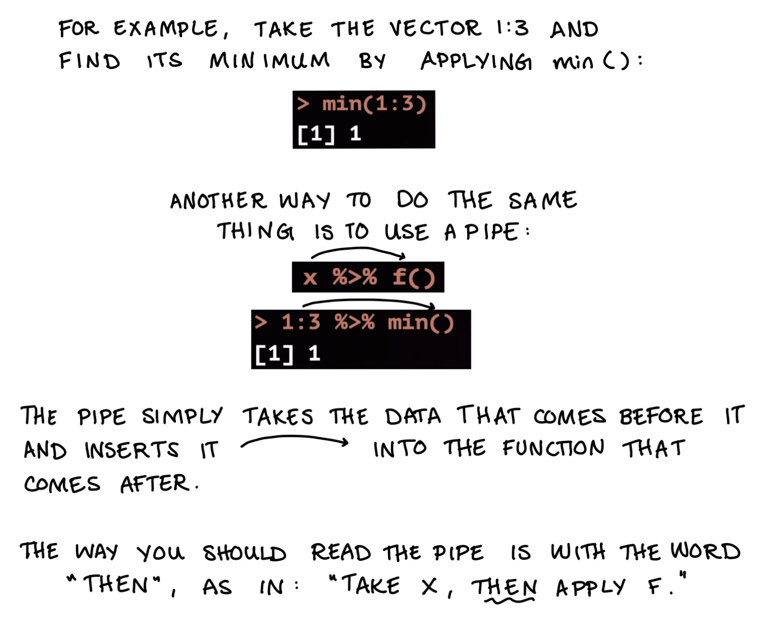
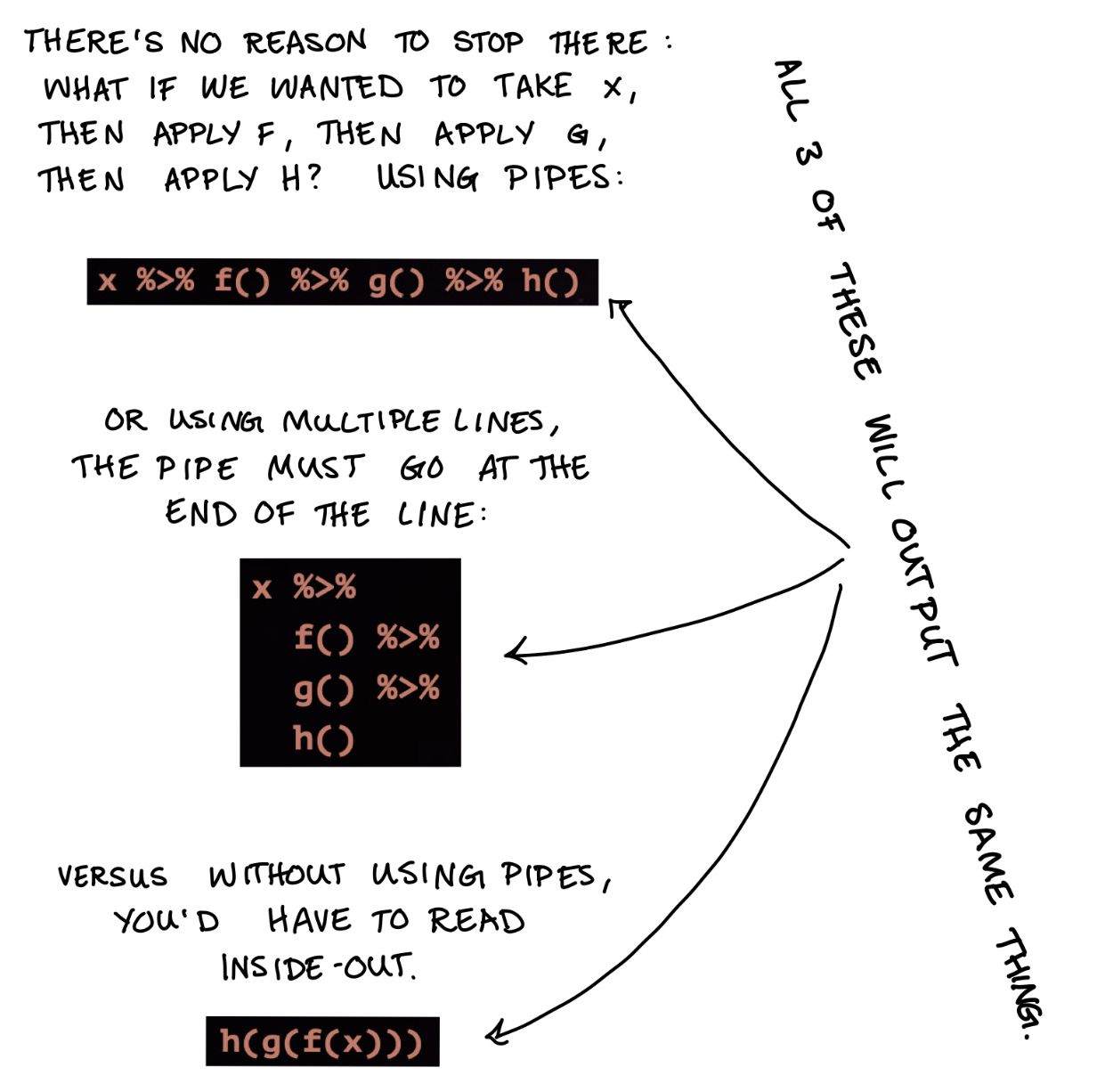
Your turn! Complete koan 3: pipes now. You’ll get practice piping data through multiple functions and combining the pipe with a period . to pipe data into the second argument of a function instead of the first.