# Example: Probability that epsilon_diff is less than -2 (probability that someone with V_diff = -2 chooses a big mac)
plogis(-2)
[1] 0.1192029A discrete choice involves selecting one option from a set of distinct alternatives. These choices can be simple, like deciding whether to buy something or not, or more complex, such as choosing between multiple options (e.g., “buy nothing,” “buy a hamburger,” “buy two hamburgers,” or “buy spaghetti”). To keep things straightforward, this assignment focuses on binary choices, where the decision-maker chooses between two options: A or B. They can’t choose both, and they can’t choose neither.
Discrete choices differ from continuous choices, which involve selecting a quantity along a continuous scale (e.g., “How many ounces of spaghetti would you like?”). Discrete variables are counted, while continuous variables are measured.
In the last unit, we used Ordinary Least Squares (OLS) to model relationships where the dependent variable was continuous, such as wage, consumption, life expectancy, or GPA. We also explored a special case where we applied OLS to a discrete dependent variable: whether or not someone won the show Love Island. In that example, we discussed how OLS estimated a linear probability model, where the model parameters represented increases or decreases in the probability of winning the show. While this approach worked, it had limitations, such as predicting probabilities outside the [0, 1] range.
In this assignment, you’ll learn about a more robust tool for modeling discrete dependent variables (also known as solving the classification problem): logistic regression, or logit for short. Unlike OLS, the logit model isn’t linear in parameters, so we’ll use a different estimation strategy called maximum likelihood estimation, which you’ll dive into in the next assignment.
In this assignment, I’ll use four greek letters:
| symbol | pronounciation |
|---|---|
| \(\alpha\) | alpha |
| \(\beta\) | beta |
| \(\varepsilon\) | epsilon |
| \(\gamma\) | gamma |
I also refer to the exponential function with \(exp()\): \(exp(x)\) means the same thing as \(e^x\) where \(e\) refers to euler’s number 2.718281…
Economists assume that decision-makers choose the option that provides the most utility. For example, if someone is deciding between a Big Mac and a chicken sandwich, they’ll choose the Big Mac if:
\[\text{Utility}_i^{big \ mac} > \text{Utility}_i^{chicken}\]
The logit model relies on the key assumption that utility functions are additively separable. This means utility can be split into an observable part (\(V\)) and an unobservable shock part (\(\varepsilon\)):
\[\text{Utility}_i^{big \ mac} = V_i^{big \ mac} + \varepsilon_i^{big \ mac}\]
\[\text{Utility}_i^{chicken} = V_i^{chicken} + \varepsilon_i^{chicken}\]
The observable part, \(V\), is a linear function of explanatory variables. For example, if age and gender tend to influence the utility someone gets from a Big Mac or a chicken sandwich, we can write:
\[V_i^{big \ mac} = \alpha_0 + \alpha_1 age_i + \alpha_2 male_i\] \[V_i^{chicken} = \gamma_0 + \gamma_1 age_i + \gamma_2 male_i\]
Exercise 1: Suppose \(\alpha_0 = 4\), \(\alpha_1 = -0.1\), \(\alpha_2 = -0.5\), \(\gamma_0 = -8\), \(\gamma_1 = 0.2\), and \(\gamma_2 = 5\). Calculate \(V_i^{big \ mac}\) and \(V_i^{chicken}\) for:
Feel free to use R to solve this problem.
If \(\varepsilon_i^{big \ mac} = 0\) and \(\varepsilon_i^{chicken} = 0\) for both people, which option will each of them choose?
The logistic regression doesn’t estimate the exact utility someone gets from each option. Instead, it estimates the difference in utility (\(V_i^{diff} = V_i^{big \ mac} - V_i^{chicken}\)) and the probability that someone with certain characteristics will choose one option over the other. In other words, it’s the relative utility that drives the decision.
An individual will choose a Big Mac if:
\[Utility_i^{big \ mac} > Utility_i^{chicken}\] That is, if:
\[V_i^{big \ mac} + \varepsilon_i^{big \ mac} > V_i^{chicken} + \varepsilon_i^{chicken}\]
Which can be rewritten as:
\[\varepsilon_i^{big \ mac} - \varepsilon_i^{chicken} > V_i^{chicken} - V_i^{big \ mac}\]
If we treat the \(\varepsilon\) terms as random variables, the probability that someone chooses a Big Mac is:
\[Prob(big \ mac)_i = Prob(\varepsilon_i^{chicken} - \varepsilon_i^{big \ mac} < V_i^{big \ mac} - V_i^{chicken})_i\]
If we make assumptions on the distribution of \(\varepsilon_i^{diff} = \varepsilon_i^{chicken} - \varepsilon_i^{big \ mac}\) and the value of \(V_i^{diff}\), we can calculate this probability. So if we want to assume that \(\varepsilon\) is normally distributed, that’s known as a probit model. For logit models, we need to assume \(\varepsilon\) follows the extreme value distribution. This assumption leads to the logistic distribution for \(\varepsilon^{diff}\), hence the name “logistic regression.”
The cumulative distribution function (CDF) for the logistic distribution is:
\[F(\varepsilon^{diff}) = \frac{exp(\varepsilon^{diff})}{1 + exp(\varepsilon^{diff})}\]
In R, you can calculate this using the plogis() function.
# Example: Probability that epsilon_diff is less than -2 (probability that someone with V_diff = -2 chooses a big mac)
plogis(-2)[1] 0.1192029Exercise 2: If \(V^{diff} = -1\) in favor of Big Macs, what is the predicted probability that someone will choose a Big Mac (assuming \(\varepsilon\) follows the extreme value distribution)? What about if someone has \(V^{diff} = 0\) in favor of Big Macs? What about if someone has \(V^{diff} = 1\) in favor of Big Macs?
The logit model maps the choice probability for all individuals based on \(V^{diff}\):
library(tidyverse)

ggplot() +
  stat_function(fun = plogis) +
  xlim(-5, 5) +
  xlab("V diff") +
  ylab("Choice Probability")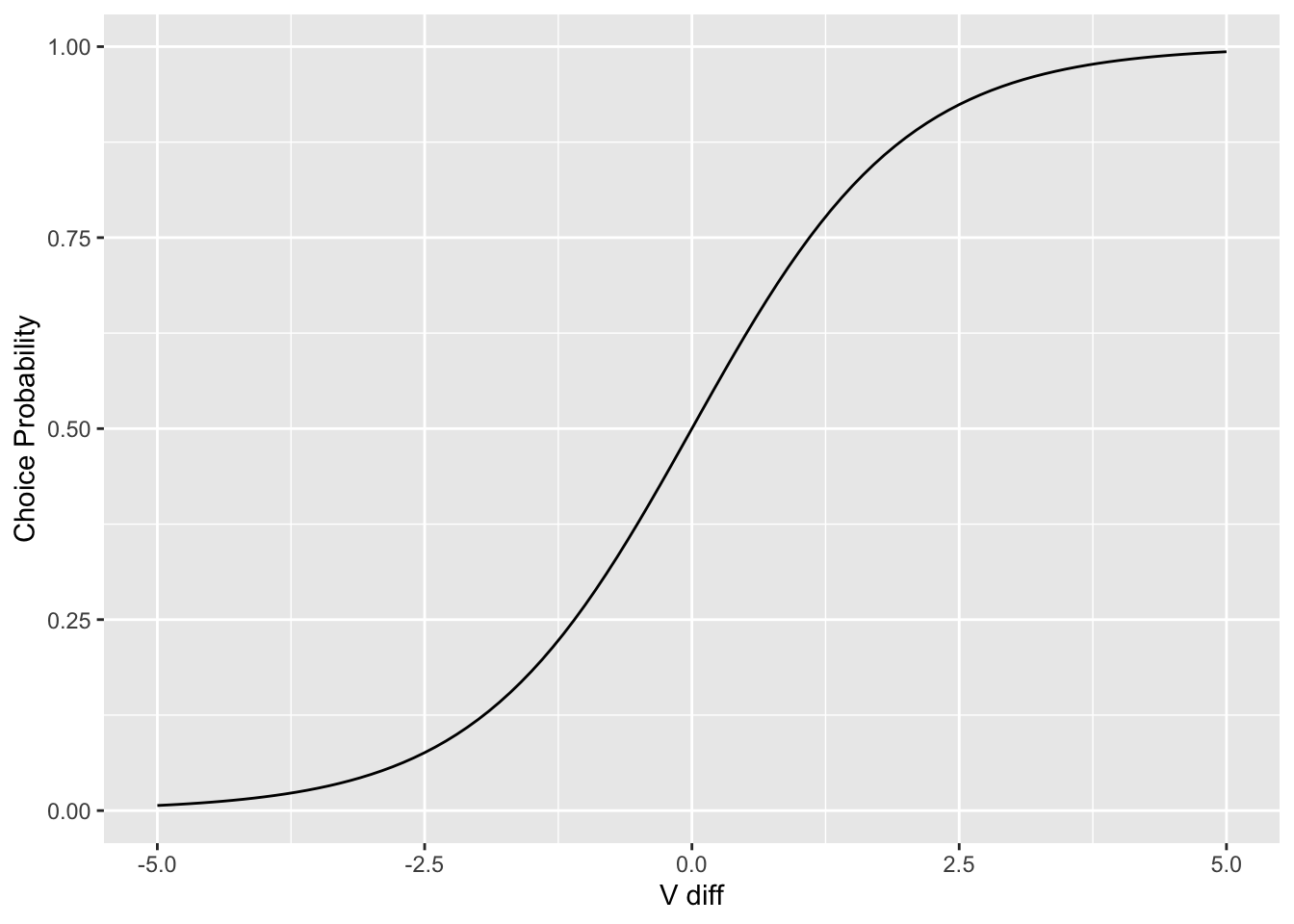
The logit choice probability is the logistic CDF evaluated at \(V_{diff}\):
\[\begin{align} Prob(big \ mac) &= F(V^{diff}) \\ &= F(\alpha_0 - \gamma_0 + (\alpha_1 - \gamma_1) age + (\alpha_2 - \gamma_2) male) \\ &= \frac{exp(\alpha_0 - \gamma_0 + (\alpha_1 - \gamma_1) age + (\alpha_2 - \gamma_2) male)}{1 + exp(\alpha_0 - \gamma_0 + (\alpha_1 - \gamma_1) age + (\alpha_2 - \gamma_2) male)} \end{align}\]
Letting \(\alpha_0 - \gamma_0 = \beta_0\), \(\alpha_1 - \gamma_1 = \beta_1\), and \(\alpha_2 - \gamma_2 = \beta_2\):
\[Prob(big \ mac) = \frac{exp(\beta_0 + \beta_1 age + \beta_2 male)}{1 + exp(\beta_0 + \beta_1 age + \beta_2 male)} \tag{17.1}\]
This model is nonlinear in parameters, so OLS can’t be used to estimate it. Instead, we’ll use maximum likelihood estimation, which you’ll learn about in the next assignment.
But what about a much simpler model of the choice probability \(Prob(big \ mac)\); one that can be estimated using OLS:
\[Prob(big \ mac) = \beta_0 + \beta_1 age + \beta_2 male + \varepsilon\]
This is called the linear probability model. I’ll discuss it, along with its shortcomings, in the next section. Then I’ll finish the chapter discussing a few more aspects of the logit.
Consider using OLS to fit this model:
\[Prob(big \ mac) = \beta_0 + \beta_1 age + \beta_2 male + \varepsilon\]
using data that looks like this:
| Big Mac (1) or Chicken Sandwich (0) | Age | Male (1) or Female (0) |
|---|---|---|
| 1 | 58 | 1 |
| 0 | 33 | 0 |
| 1 | 17 | 0 |
| 0 | 23 | 1 |
| 1 | 59 | 1 |
Interpreting this data: the first person is a 58 year old male who buys a big mac. The second person is a 33 year old female who buys a chicken sandwich.
One option would be to use OLS. Here I load an artificial dataset and visualize this model. Notice I use geom_jitter() instead of geom_point() because the overplotting would make the plot very hard to understand:
library(tidyverse)

set.seed(1234)

# Here I generate some artificial logit data:
data <- tibble(
  # Let ages be between 16 and 65
  age = sample(16:65, replace = T, size = 1000),
  male = sample(0:1, replace = T, size = 1000),
  # The (observable) value someone gets from a big mac depends on their age and sex:
  v = 2 - .1 * age + 2.8 * male,
  # The probability they buy a big mac depends on v according to the logit:
  prob_big_mac = exp(v) / (1 + exp(v)),
  # They buy a big mac with the probability prob_big_mac.
  big_mac = rbinom(n = 1000, size = 1, prob = prob_big_mac)
) %>%
  mutate(male = as.factor(male))
data %>%
ggplot(aes(x = age, y = big_mac, color = male)) +
geom_jitter(height = .15) +
geom_smooth(method = lm)`geom_smooth()` using formula = 'y ~ x'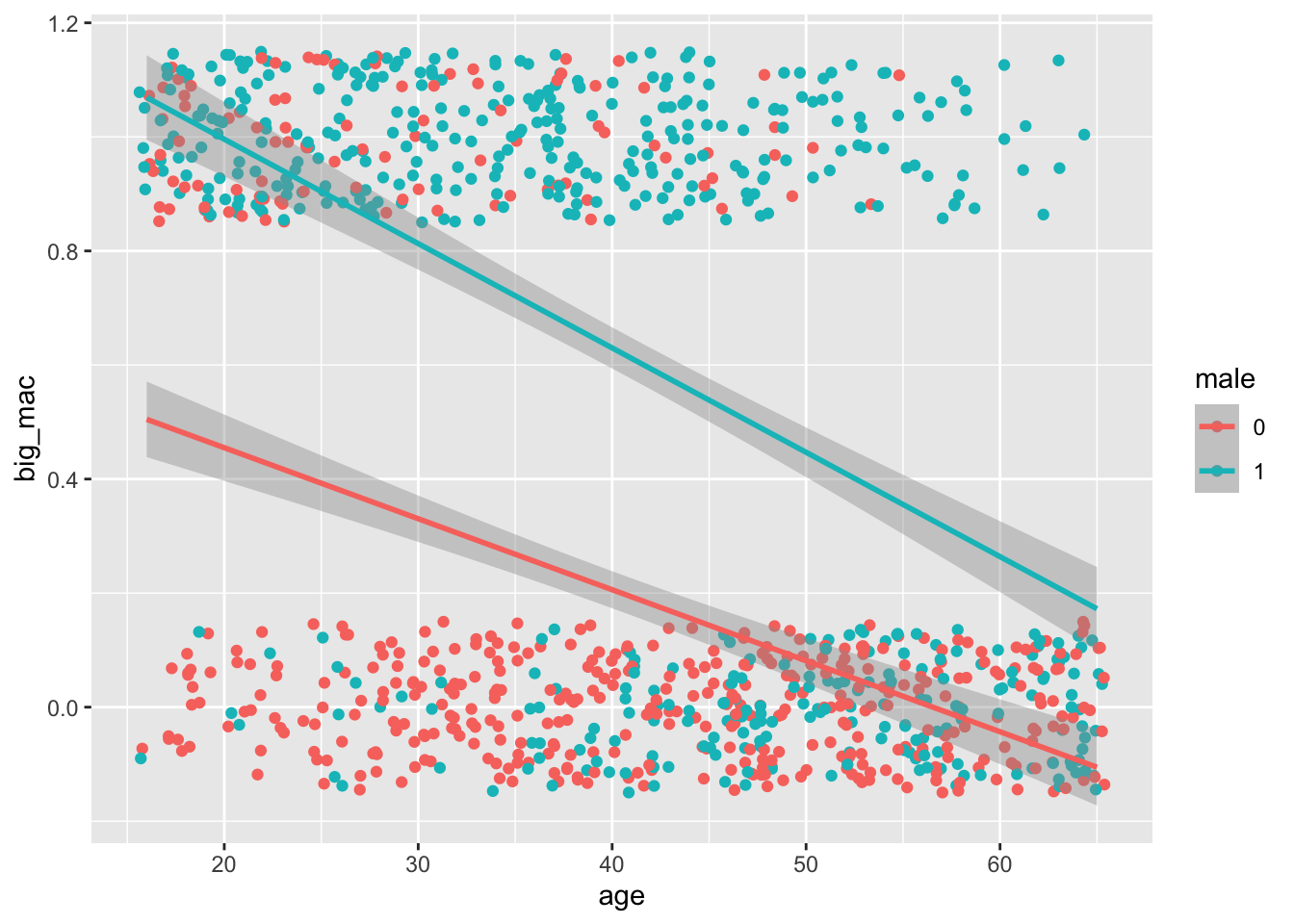
lm(big_mac ~ age + male, data = data) %>%
    broom::tidy(conf.int = TRUE)
# A tibble: 3 × 7
term estimate std.error statistic p.value conf.low conf.high
<chr> <dbl> <dbl> <dbl> <dbl> <dbl> <dbl>
1 (Intercept) 0.826 0.0408 20.3 9.70e-77 0.746 0.906
2 age -0.0155 0.000908 -17.0 2.54e-57 -0.0173 -0.0137
3 male1 0.421 0.0249 16.9 1.78e-56 0.372 0.470 This is called a linear probability model because it’s linear in parameters and you can interpret the fitted values for big_mac as the probability that someone will buy a big mac over a chicken sandwich given their age and gender.
Exercise 3: Interpret the estimates for this linear probability model. In particular, what’s the estimated probability that a 16 year old male will buy a big mac? And what’s the estimated probability a 50 year old female will buy a big mac?
There are two big problems with this linear probability model:
Estimated probabilities can easily be less than 0 or greater than 1, which makes no sense for probabilities. Nothing about OLS guarantees that the fitted values are reasonable numbers for probabilities.
We’ve assumed the relationship between the explanatory variables and the probability someone buys a big mac over a chicken sandwich is linear, but this might not reflect reality. We’d probably prefer a model that lets marginal effects change: for example, maybe going from age 15 to age 25 doesn’t change the probability you’ll buy a big mac very much, but going from age 45 to 55 creates a much larger behavioral change.
Guess what: the logit solves both these problems: instead of \(Prob(\ big \ mac_i)\) on the left hand side, we’ll have the log odds of buying a big mac on the left hand side. Odds are just the probability you do the thing divided by the probability you don’t.
\[log_e \left (\frac{Prob(big \ mac)_i}{Prob(chicken)_i} \right ) = \beta_0 + \beta_1 age_i + \beta_2 male_i\]
And because you either buy a big mac or you buy a chicken sandwich, \(Prob(chicken) = 1 - Prob(big \ mac)\) so the logit is also:
\[log_e \left (\frac{Prob(big \ mac)_i}{1 - Prob(big \ mac)_i} \right ) = \beta_0 + \beta_1 age_i + \beta_2 male_i\]
Exercise 4: Show that if you take the model above and solve for \(Prob(big \ mac)\), you’ll get that: \[Prob(big \ mac)_i = \frac{exp(\beta_0 + \beta_1 age_i + \beta_2 male_i)}{1 + exp(\beta_0 + \beta_1 age_i + \beta_2 male_i)}\] Which is exactly the way I defined the logit in Equation 17.1.
Exercise 5: A logit will never predict a probability outside of the \((0, 1)\) range. Show that this is true using the formula from Equation 17.1. In particular, consider what \(Prob(big \ mac)_i\) will be if \(\beta_0 + \beta_1 age_i + \beta_2 male_i\) is very large, like 1,000,000, or very negative, like -1,000,000.
Take \(\beta_0 = -2\) and \(\beta_1 = .05\) for a logit with just one explanatory variable. We can take the formula \(Prob(option \ A)_i = \frac{exp(\beta_0 + \beta_1 x_i)}{1 + exp(\beta_0 + \beta_1 x_i)}\) and plot \(Prob(option \ A)\) on the y-axis against the explanatory variable x on the x-axis:
tibble(
    x = 0:100,
    p = exp(-2 + .05 * x) / (1 + exp(-2 + .05 * x))
) %>%
    ggplot(aes(x = x, y = p)) +
    geom_line()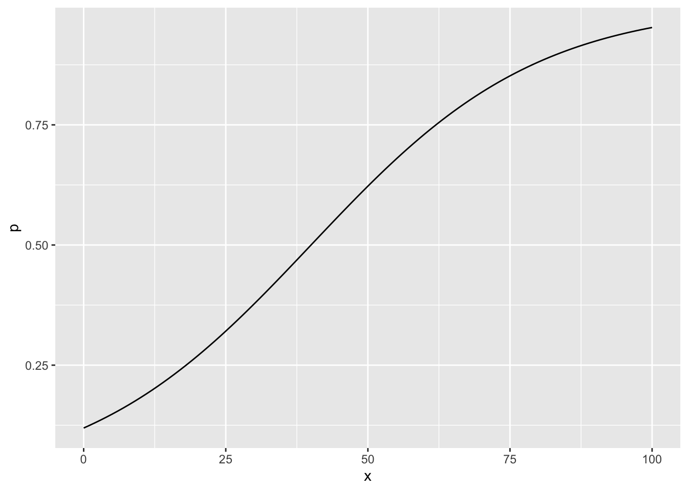
The plot above shows that marginal effects for logits can vary. Here, they start small, increase, and then decrease (I’m looking at the slope of the curve above). That is, going from x = 15 to 25 creates a small increase in the probability you’ll take option A over option B, but not as much as the behavioral change going from x = 40 to 50. And by the time x = 90 or 100, the marginal impact of x on the probability you’ll take option A is small again (perhaps because everyone possibly interested in taking option A is already taking it).
To interpret the coefficients \(\hat{\beta_0}\) and \(\hat{\beta_1}\) for a logit, consider the model again:
\[log_e \left (\frac{p(y_i = 1)}{1 - p(y_i = 1)} \right ) = \beta_0 + \beta_1 x_i\]
\(\hat{\beta_0}\) is the estimated log odds of “a success” given x = 0. \(\hat{\beta_1}\) is the estimated increase in the log odds of a success when x increases by 1 unit.
I’ll use glm() to fit the logit for the big mac example using artificial data. I’ll discuss a little of what’s going on behind the scenes to fit this model in the next chapter on maximum likelihood estimation.
glm(big_mac ~ age + male, data = data, family = "binomial") %>%
  broom::tidy(conf.int = TRUE)
# A tibble: 3 × 7
term estimate std.error statistic p.value conf.low conf.high
<chr> <dbl> <dbl> <dbl> <dbl> <dbl> <dbl>
1 (Intercept) 2.10 0.265 7.95 1.91e-15 1.59 2.63
2 age -0.0981 0.00737 -13.3 2.03e-40 -0.113 -0.0840
3 male1 2.56 0.190 13.5 2.62e-41 2.20 2.94 Exercise 6: Interpret these estimates by answering: what is my estimate for the probability that a 20 year old male will get a big mac? And what about a 50 year old female?
Finally, I’ll visualize the logit I just estimated:
data %>%
    ggplot(aes(x = age, y = big_mac, color = male)) +
    geom_jitter(height = .15) +
    stat_smooth(method = "glm", se = FALSE, method.args = list(family = binomial))
`geom_smooth()` using formula = 'y ~ x'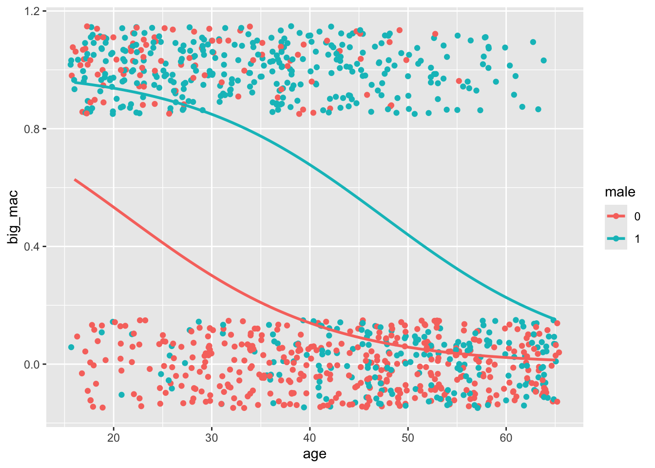
Exercise 7: Go to Project Euler and create an account. Doing this will let you check your answer to the problems you’re about to do. Then go to Archives and solve problem 1: If we list all the natural numbers below 10 that are multiples of 3 or 5, we get 3, 5, 6 and 9. The sum of these multiples is 23. Find the sum of all the multiples of 3 or 5 below 1000. Your imperative programming toolkit is below.
You’re already comfortable with most of these operators, so here’s just a quick refresh.
+ - * / ^
# Addition and subtraction
1 + 1
[1] 21 - 1[1] 0# Multiplication and division
1 * 2[1] 24 / 2[1] 2# Exponents
2 ^ 3[1] 8These two are also very useful: %% and %/%
# This operator: %% finds the remainder if you divide two numbers.
# Since 2 goes into 10 evenly, the remainder is 0:
# You'd say that "10 mod 2 is 0:"
10 %% 2
[1] 0# This operator: %/% does integer division: 3 goes into 10 3 times.
10 %/% 3[1] 3== != > < >= <= & |
# 3 "is equal to" 3
3 == 3
[1] TRUE# 3 "is not equal to" 2
3 != 2[1] TRUE# 3 "is greater than" 2
3 > 2[1] TRUE# 3 "is greater than or equal to 2"
3 >= 2[1] TRUE# 3 is greater than 2 "AND" 4 modulo 2 is 0:
(3 > 2) & (4 %% 2 == 0)[1] TRUE# 3 is greater than 2 "OR" 4 modulo 3 is 0:
(3 > 2) | (4 %% 3 == 0)[1] TRUEHere’s an example of an if statement inside of a function that checks to see if a number x is larger than 3. If it is, it prints a statement.
larger_than_3 <- function(x) {
    if (x > 3) {
        print("This number is larger than 3")
    }
}

larger_than_3(5)
[1] "This number is larger than 3"# It does nothing if x is not larger than 3.
larger_than_3(2)You could use an if/else ladder if you wanted there to be more than one condition. You could also have your function return a character string instead of just a side effect of printing it.
sign <- function(x) {
    if (x > 0) {
        return("positive")
    } else if (x == 0) {
        return("zero")
    } else {
        return("negative")
    }
}

sign(5)
[1] "positive"sign(0)[1] "zero"sign(-5)[1] "negative"The first programmers had only mathematical operators, if for making comparisons, and jump statements that would let them skip sections of code depending on a logical condition. Somewhere along the line, they realized jump statements made code impossible to read and understand. Someone offered a solution: for and while loops. They’re just simple patterns that became really popular because they helped people write clearer programs.
Here’s an example of a for loop inside of a function (with an if statement!). It prints even numbers less than or equal to any number x. It has an iterating variable i that iterates through the sequence 1:x, checking whether the number i is evenly divisible by 2, and if it is, it prints i.
evens_less_than <- function(x) {
    for (i in 1:x) {
        if (i %% 2 == 0) {
            print(i)
        }
    }
}

evens_less_than(10)
[1] 2
[1] 4
[1] 6
[1] 8
[1] 10While loops are just like for loops, except instead of iterating through a sequence, they iterate until the logical condition fails to hold. This function prints all the numbers less than a certain number x. It initiates y at 0 and then as long as y continues to be less than x, it keeps on printing y and then adding 1 to y.
numbers_less_than <- function(x) {
    y <- 0
    while(y < x) {
        print(y)
        y <- y + 1
    }
}

numbers_less_than(5)
[1] 0
[1] 1
[1] 2
[1] 3
[1] 4If you’re working with a vector, you can use bracket notation to select certain elements of that vector:
# The first element of this vector can be selected using [1]:
c(1, 2, 3)[1]
[1] 1# The first two elements of this vector can be selected using [1:2]:
c(1, 2, 3)[1:2][1] 1 2Likewise, if you’re working with a 2d data structure like a matrix, you can use bracket notation to select a certain row, column element:
m <- matrix(1:9, nrow = 3)

print(m)
[,1] [,2] [,3]
[1,] 1 4 7
[2,] 2 5 8
[3,] 3 6 9# Select the first row and first column
m[1, 1][1] 1# Reassign the first row and first column
m[1, 1] <- 10
print(m) [,1] [,2] [,3]
[1,] 10 4 7
[2,] 2 5 8
[3,] 3 6 9$ for extracting a vector from a tibble (tidyverse uses pull())You can use $ to take a tibble like gapminder and extract a column vector like lifeExp. l is now a vector:
library(gapminder)

l <- gapminder$lifeExp

l[1:5]
[1] 28.801 30.332 31.997 34.020 36.088