5 Supply and Demand – Economics of Organizations

5.1 Variable Pricing and Demand

In 2003, the Colorado Rockies began using variable pricing to boost revenue without increasing costs for season-ticket holders. Variable pricing means charging different prices for the same seat based on factors like the opponent or game day. This practice, common at the time in hotels and concert venues, was soon adopted across MLB. Teams started charging more for popular games and lowering prices during losing streaks to attract fans. The Giants reported that variable pricing helped them sell 25,000 extra tickets in 2009 and increased their revenue by $500,000.

MLB teams now use sophisticated computer models to analyze past ticket sales and data from secondary markets to set ticket prices based on estimated market demand. These models consider a large number of variables, such as day of the week, team performance, and pitching matchups, to predict the optimal ticket price for each seat and game. The models assign weights to each variable, reflecting its influence on demand. The result is a dynamic pricing strategy that adjusts ticket prices to maximize revenue while reflecting real-time market conditions.

5.2 The Demand Side of a Market

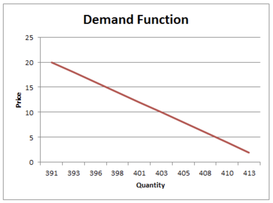
The quantity of a good that people demand depends on various factors, including their income, preferences, the prices of substitutes and complements, advertising efforts, and the quality of the product and its alternatives. A demand function captures the relationship between price and quantity demanded at a specific moment, assuming all these factors remain constant. Typically, demand curves slope downward—a helpful way to remember this is that both “demand” and “down” start with “d.” This downward slope reflects the idea that as the price of a good falls, sales usually increase.

However, if any of these influencing factors change, the demand curve shifts. For instance, when people’s incomes rise, they tend to buy more baseball tickets at any given price, meaning there is a rightward shift in the demand curve for baseball tickets when incomes increase.

5.3 The Supply Side of a Market

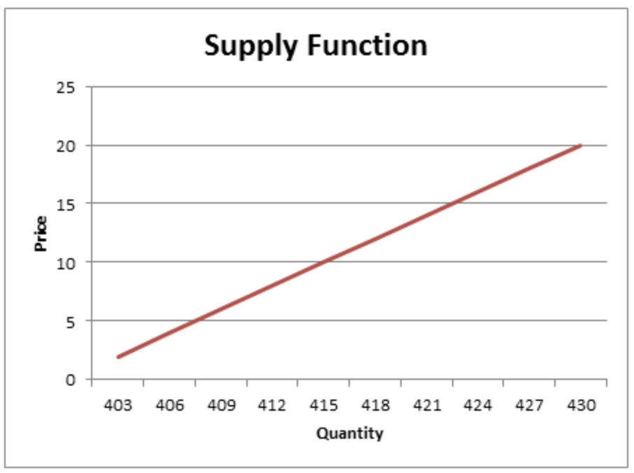
The market supply curve illustrates the number of units sellers are willing to offer at various prices. Typically, supply curves slope upward, meaning that higher prices provide incentives for suppliers to produce more. A simple way to remember this is that “up” is part of the word “supply.”

The position of the supply curve is influenced by factors such as production technology and the cost of inputs like labor, capital, and land. When a more cost-effective production technology is introduced, suppliers can offer more units at every given price, causing the supply curve to shift to the right. Conversely, if the cost of labor rises, suppliers may offer fewer units at each price point, leading to a leftward shift of the supply curve.

5.4 Equilibrium

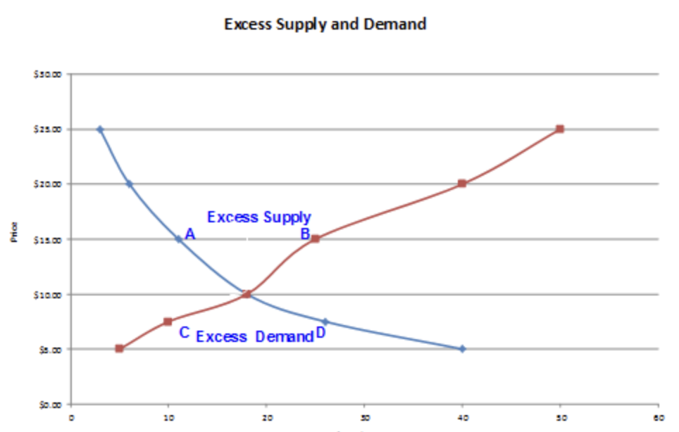
Economists represent markets as the interaction between demand and supply curves. By overlaying the supply curve on the demand curve, we can analyze how changes in prices affect the market balance. If the price is set above the point at which the demand and supply curves intersect, the quantity supplied will exceed the quantity demanded, leading to excess supply. Producers with unsold inventories may be forced to lower their prices to clear their stock, making such a high price unsustainable in the long run.

On the other hand, if the price is below the intersection point, the quantity demanded exceeds the quantity supplied, resulting in a shortage. Consumers eager to buy may struggle to find sellers, prompting suppliers to raise their prices. Therefore, a price below the intersection is also unsustainable.

The sustainable market price is found at the intersection of the demand and supply curves, where the quantity demanded equals the quantity supplied. At this price, the market is balanced: every buyer can find a seller, and every seller can find a buyer. This state of balance is referred to as market equilibrium.

5.5 Classwork 5

Suppose you were given the following information about the market demand for a good:

Price	Quantity Demanded
14	0
13	1
12	2
11	3
10	4
9	5
8	6
7	7
6	8
5	9
4	10
3	11
2	12
1	13
0	14

Price	Quantity Supplied
2	0
3	1
4	2
5	3
6	4
7	5
8	6
9	7
10	8
11	9
12	10
13	11
14	12

Predict market equilibrium using several methods:

5.6 A) Graphically:

Using R, put the data into two tibbles, one called demand and one called supply. Draw a plot using ggplot() and try to eyeball where the supply and demand lines cross.

Give your supply and demand curves different colors. R offers 657 color names, and you can read all of them using the command colors().

library(tidyverse)

demand <- ___

supply <- ___

demand %>%
  ggplot(___) +
  geom_line(___) +
  geom_line(___)

5.7 B) Numerically

In equilibrium, we know that excess supply (and excess demand) is zero. Use R to join your two tibbles and then use dplyr to add a new column representing either excess supply or excess demand. For what values of price and quantity is excess supply equal to zero? Do these numbers agree with your answer to part a?

demand %>%
  left_join(___) %>%
  mutate(___) %>%
  filter(___)

5.8 C) Algebraically

Use lm() to find the equations of the lines of best fit for supply and demand. In equilibrium, we know that quantity supplied is equal to quantity demanded, so you can set expressions equal to each other and solve for $q$ and $p$. Do these numbers agree with your answers in parts a and b?

demand %>% lm(___)

supply %>% lm(___)

5.9 D) Using dplyr and ggplot, show what happens to price and quantity exchanged when there is an increase in supply (that is, firms are willing to supply more at any given price).

supply %>%
  mutate(___) %>%
  ggplot(___) +
  geom_line(___) +
  geom_line(___) +
  geom_line(___) +
  annotate("text", x = 10.5, y = 11, label = "Supply Shift", color = "salmon", vjust = -1) +
  annotate("segment", x = 9, xend = 12, y = 11, yend = 11, color = "salmon", arrow = arrow(type = "closed", length = unit(0.2, "inches")))

:::