13 Scale and Scope Economies – Economics of Organizations

13.1 Classwork 12 Review Questions

13.2 Long-Run Average Cost Functions

In the long run, all inputs are variable, allowing producers to choose any size or type of production facility. Since no inputs are fixed, there are no fixed costs in the long run. This flexibility enables producers to operate as efficiently as possible.

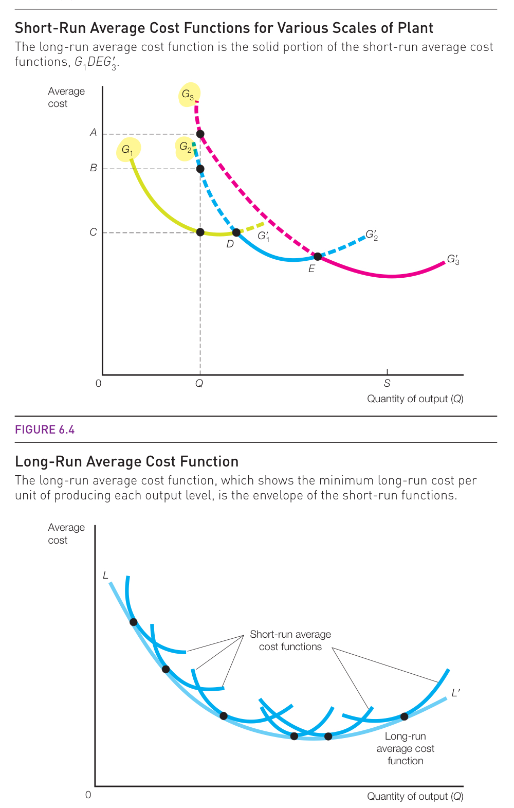
For example, consider a producer deciding whether to build 1, 2, or 3 factories. Building just one factory is the most cost-effective way to produce a small amount of output. However, as the desired output increases, it eventually becomes cheaper (in terms of average costs) to build two factories rather than overworking a single factory. In the figure below, $G_1$ represents the short-run average cost curve for one factory, $G_2$ for two factories, and $G_3$ for three factories. The long-run average cost curve is the minimum of these short-run average cost curves because, in the long run, producers have the flexibility to be the most efficient they can possibly be, and therefore would never choose a higher cost plant scale when one with a lower cost is also available.

13.3 Economies of Scale

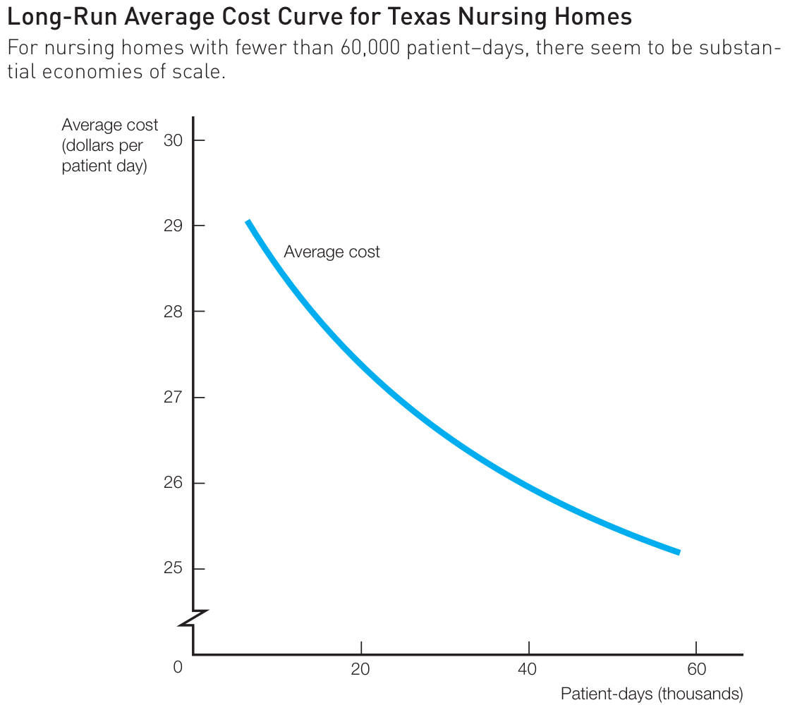
A long-run average cost curve represents the relationship between ouput $Q$ and average costs. Consider this average cost curve for nursing homes:

This shows that nursing homes have an economy of scale: the more residents they have, the lower the cost per resident. There are lots of reasons a producer could experience an economy of scale (average cost savings as quantity increases): bulk purchasing, spreading fixed costs, distribution networks, etc. The size of cruise ships keep growing because larger ships have a lower cost per passenger thanks to scale economies.

But at some point, every average cost curve eventually slopes back upward (experiencing a diseconomy of scale). Eventually, a large enough company becomes too complicated to manage efficiently. Communication becomes difficult, there is increased administrative overhead, and efforts become duplicated.

Economy of Scale: when the firm’s average unit cost decreases as output increases.

Diseconomies of Scale: when the average costs per unit of output increase.

13.4 Economies of Scope

Economies of scale are not the only cost-saving strategy for producers. Consider a company that produces both shampoo and conditioner. Instead of having two separate production lines for each product, the company can use the same factory, distribution network, marketing team, and even some common ingredients (like packaging materials and fragrances) to produce both products. This reduces the average cost of production for each item because shared resources (like the factory space and marketing campaigns) are spread across both products, rather than each having its own entirely separate set of costs.

Economies of Scope: Exist when the cost of jointly producing two or more products is less than the cost of producing each one alone.

Of course, there are also diseconomies of scope. Diseconomies of scope can occur when a company adds a new product line that harms its brand or requires significant investment in new production facilities and expertise. This could lead to higher average costs than if the two products were produced by entirely separate companies.

13.5 Classwork 13: Short-Run vs Long-Run Cost Functions

Hints for this classwork:
- In the short run, both labor ($L$) and capital ($K$) are fixed.
- In the long run, (circle one: all inputs/no inputs) are fixed.
- Total costs increase with output $Q$. The average cost function is equal to total costs per unit of output: $\frac{TC}{Q}$. Marginal costs are the change in costs for an extra unit of output: $\underline{\hspace{2cm}}$.
- Suppose you have a function $f(x)$ and you want to find its minimum. At the minimum, the slope of the tangent line is equal to $\underline{\hspace{2cm}}$, so you can find where $f'(x) = 0$. You should also check the second derivative to make sure you haven’t found a maximum instead: $f''(x) > 0$ for (minima/maxima) and $f''(x) < 0$ for (minima/maxima).
- The Cobb-Douglas shortcut says that when you have Cobb-Douglas utility (production) that’s of the form $c x_1^a x_2^b$, where $a + b = 1$, you’ll spend $\underline{\hspace{2cm}}$ of your income (total cost) on good 1 (input 1), and you’ll spend $\underline{\hspace{2cm}}$ of your income (total cost) on good 2 (input 2). So if your income is $m$ and good 1 has a price of $p_1$, $x_1 p_1 = m a$ and solving for $x_1$, we get that $x_1 = \frac{ma}{p_1}$.
Suppose a producer’s production function is given by $Q = 4 K^.5 L^.5$, where $Q$ is the output (in thousands of units per month), $L$ is the number of hours of labor employed per month (in thousands), and $K$ is the capital used per month (in thousands of units). Suppose workers are paid $8 an hour and capital costs $2 per unit. The total cost function is therefore: $TC = \underline{\hspace{1cm}} L + \underline{\hspace{1cm}} K$.
The Cobb-Douglas shortcut says that in order to minimize costs subject to a certain level of output, the producer will choose $K = \underline{\hspace{1cm}} TC$ and $L = \underline{\hspace{1cm}} TC$.
Use the production function to eliminate $L$ and derive a function of total cost that expresses a relationship between total cost and the quantity of output produced $Q$. That is, show that $TC = \frac{Q^2}{2K} + 2K$.
In the short-run, suppose labor and capital are fixed such that $K = 10$. Continue from part d) to find (short-run) $TC$ as a function of only $Q$.
Calculate the short-run average cost function.
Calculate the short-run marginal cost function.
Verify: when $MC = AC$, is $AC$ minimized? Explain the intuition about why this is always the case.
In the long-run, the producer can choose any ouput level $Q$ and determine $L$ and $K$ to be able to produce that output level at the minimum total cost. Take this $TC$ equation: $TC = \frac{Q^2}{2K} + 2K$ and find the value of $K$ which minimizes the $TC$, treating $Q$ as a constant.
Use your answer to part h) to find the producer’s cost minimizing choice for $L$.
Finally, compare your answers from parts i) and j) to your hypothesis in part c). Have you verified that the Cobb-Douglas shortcut works to find the long-run cost minimizing input bundle?