library(tidyverse)

data <- tibble(
    price = 5:10,
    quantity = c(41, 44, 49, 80, 59, 42)
)

data %>%
    ggplot(aes(x = quantity, y = price)) +
    geom_point(size = 3)
For more information on these topics, see Allen, Doherty, Weigelt, and Mansfield Chapter 4: Estimating Demand Functions.
Demand elasticity helps us understand market power by showing how sensitive consumers are to price changes. If demand is elastic, businesses have less power to raise prices without losing customers, but if it’s inelastic, they can charge more without losing many sales. This is important for studying how companies influence prices and compete in markets. Economists therefore need ways to reliably estimate demand elasticities, but the challenge is that there’s an identification problem. This chapter explains what that problem is and how to get around it.
So far, we’ve discussed the “Marshallian Cross” model of the determination of market prices. The demand curve slopes down and the supply curve slopes up, and the equilibrium price and quantity exchanged are at the intersection of those two curves. So if you had data on prices and quantities exchanged and you ran a regression like this one: lm(q ~ p), would you be estimating the supply curve or the demand curve? The answer is neither, because of the simultaneous equation bias.
Practice Question: Why can’t you estimate the demand or supply curve using the regression model lm(q ~ p) with data on prices and quantities exchanged of a good?
Consumer demand is determined by consumer indifference curves and budget constraints. Indifference curves come from consumer tastes, which can be influenced by advertising. Consumer budget constraints depend on incomes \(m\) and the prices of other goods, especially if they are substitutes or complements with the good in question.
Practice Question: Advertising can influence consumer demand by shifting:
Practice Question: If two goods are complements, how would an increase in the price of one good affect the consumer’s demand for the other good?
We’ll discuss the determinants of supply in the next few chapters, but as a preview, supply is determined by things like: production costs, technology, the number of sellers in the market, and expectations of future prices.
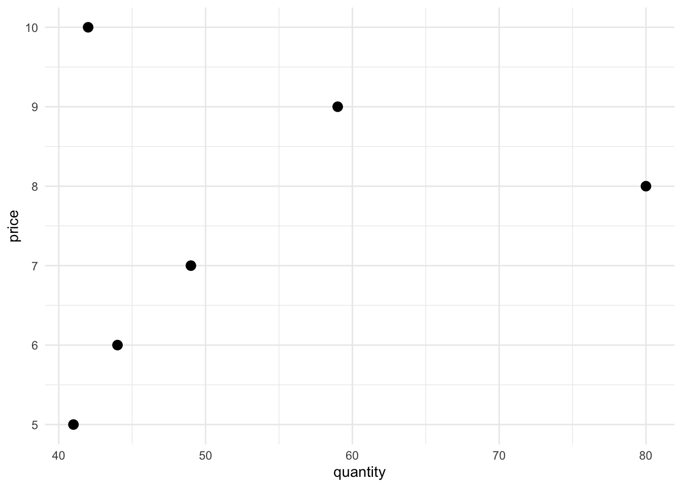
Consider the following data:
library(tidyverse)
data <- tibble(
price = 5:10,
quantity = c(41, 44, 49, 80, 59, 42)
)
data %>%
ggplot(aes(x = quantity, y = price)) +
geom_point(size = 3)
Suppose I told you that no determinants of supply or demand changed the entire time this data was collected. That is, consumer tastes, incomes, and the prices of other goods stayed the same. And production costs, technology, the number of sellers in the market, and expectations of future prices all stayed the same as well. Then you’d have to chalk up the observed variations in price and quantity exchanged to randomness. The data would give you no useful information about estimating the supply or demand curves.
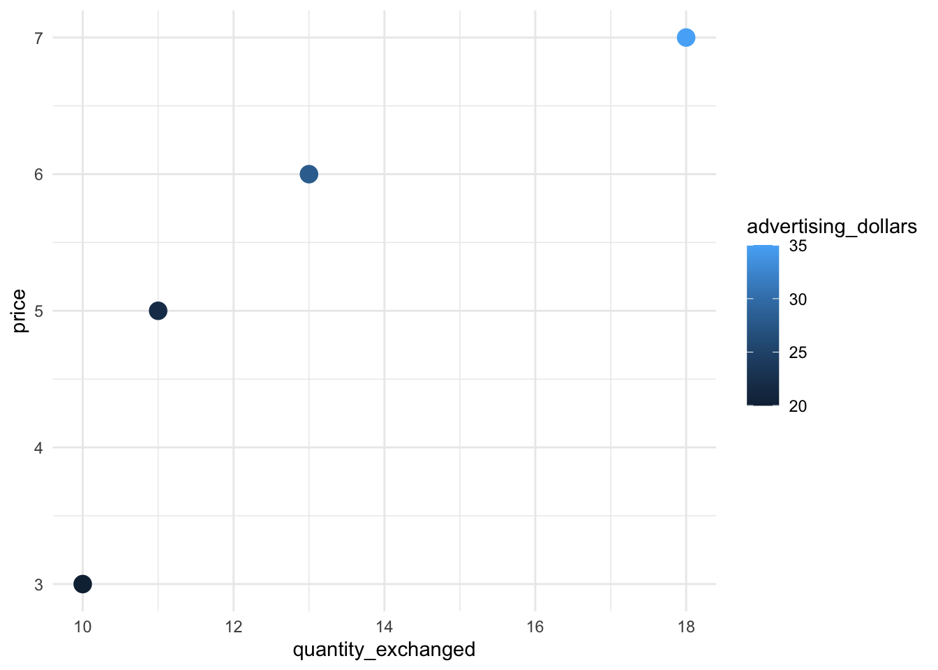
But if I told you that no determinants of supply or demand changed the entire time this data was collected except for advertising dollars spent by the producer, that’s a different story.
data <- tibble(
    price = c(3, 5, 6, 7),
    quantity_exchanged = c(10, 11, 13, 18),
    advertising_dollars = c(20, 22, 28, 35)
)

data %>%
    ggplot(aes(x = quantity_exchanged, y = price, color = advertising_dollars)) +
    geom_point(size = 4)
data %>%
    ggplot(aes(x = quantity_exchanged, y = price, color = advertising_dollars)) +
    geom_point(size = 4) +
    geom_smooth(method = lm, se = F)
`geom_smooth()` using formula = 'y ~ x'
data %>%
    lm(quantity_exchanged ~ price, data = .)
Call:
lm(formula = quantity_exchanged ~ price, data = .)

Coefficients:
(Intercept)        price
      3.400        1.829
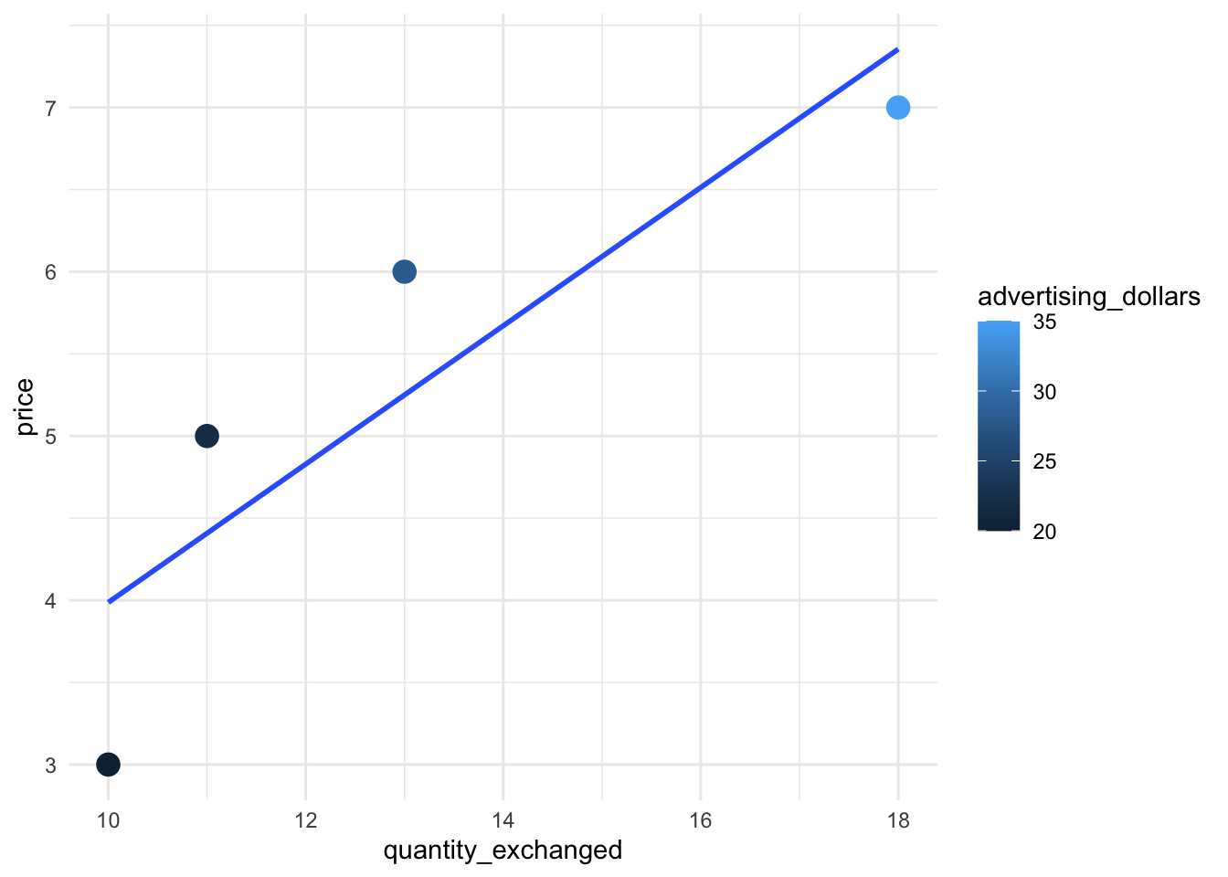
And so, we have an estimate for the supply function:
\(q(p) = 3.4 + 1.8 p\)
And of course we could also fit a constant elasticity supply curve model instead of a linear one:
data %>%
    ggplot(aes(x = quantity_exchanged, y = price, color = advertising_dollars)) +
    geom_point(size = 4) +
    geom_smooth(method = glm, se = F, method.args = list(family = gaussian(link = "log")))
`geom_smooth()` using formula = 'y ~ x'
data %>%
    lm(log(quantity_exchanged) ~ log(price), data = .)
Call:
lm(formula = log(quantity_exchanged) ~ log(price), data = .)

Coefficients:
(Intercept)   log(price)
     1.5749       0.5983
Which says our model has this fit:
\[\log(q) = 1.57 + 0.60 \log(p)\]
Or in other terms,
\[q = e^{1.57} p^{0.60}\]
Which indicates that supply has a constant elasticity of 0.60, which is fairly inelastic. Producers can’t easily escape the market.
Practice Question: If you have data on price, quantity exchanged, and advertising dollars, and you assume all supply determinants stayed steady over the period in question, you can use a linear regression to estimate:
We’ll continue to explore these topics in Classwork 9.
Some R prerequisites:
You can generate a vector of numbers that are drawn from the normal distribution using the function rnorm(). That function takes a number of observations to generate (default is n = 1), a mean (default is mean = 0), and a standard deviation (default is sd = 1). Learn more about this function by reading the help docs: ?rnorm. Use rnorm() to generate 100 random normal numbers with mean 0 and standard deviation 1.
You can generate a vector of numbers that are drawn from a random uniform distribution using the function runif(). That function takes a number of observations to generate (there is no default), a minimum value (default is min = 0), and a maximum value (default is max = 1). Generate 1000 random uniform numbers between 70 and 80.
When you create a tibble, you can make one variable be a function of other variables. For example: use tibble() to generate a variable x which is a vector of 10 random normals. Let y be x multiplied by 10.
tibble(
    x = ___,
    y = ___
)
In the workbook, you learned that if you have data about prices and quantities exchanged, you can use it to estimate (choose one: the supply curve; the demand curve; neither the supply nor the demand curves) because \(\underline{\hspace{2cm}}\).
You also learned that if you’re willing to assume that none of the supply determinants changed during the data collection period (supply determinants include \(\underline{\hspace{2cm}}\)), but some of the demand determinants did change (demand determinants include \(\underline{\hspace{2cm}}\)), then you can use the data to run the regression lm(q ~ p) to estimate the \(\underline{\hspace{2cm}}\) curve.
In this classwork, you’ll simulate the opposite scenario: if you assume that none of the demand determinants changed, but some of the supply determinants did, then you can use the data to run the regression lm(q ~ p) to estimate the \(\underline{\hspace{2cm}}\) curve.
Suppose that the demand curve is \(q(p) = 14 - p\) and that the supply curve is \(q(p) = 2 + p - w\), where \(w\) refers to the wage rate of workers. The demand curve indicates that consumers are willing to buy (choose one: more/fewer) units of the good as the price increases. The supply curve indicates that producers are willing to supply (choose one: more/fewer) units of the good as the price increases. The supply curve also indicates that producers are willing to supply (choose one: more/fewer) units of the good as the wage rate of workers increases.
Continuing from part e), solve for the equilibrium price as a function of only the wage rate.
Again continuing from part f), generate a synthetic dataset called market that has three variables: w, p, and q, and 1000 rows. Define them this way: the wage rate w should be random uniform between 5.5 and 20. Define p using the equation you found in part f: these are equilibrium prices given a wage rate. Define q using either the supply or demand equations (it will come out the same either way), and add a vector of 1000 random normals (mean 0, standard deviation 1) to represent some random noise.
Take market and visualize the equilibrium prices and quantities using a scatterplot.
Take market and estimate the model \(q = \beta_0 + \beta_1 p + u\) using lm(q ~ p). What were the true values in the data generating process for the model parameters? Is your estimation close?