15 Long-run Equilibrium in Perfectly Competitive Markets
For more information on these topics, see Allen, Doherty, Weigelt, and Mansfield Chapter 7: Perfect Competition.
In perfectly competitive markets, individual decisions by firms and consumers lead to efficient outcomes over time, as if guided by an “invisible hand.” Let’s explore how these markets adjust in the long run.
15.1 Profit Maximization: MR = MC
A firm’s profit is its total revenue minus its total cost. All firms aim to maximize their profit by producing where marginal revenue (\(MR\)) equals marginal cost (\(MC\)). In perfect competition, firms are price takers, so \(MR\) equals the market price for all units.
Imagine you’re running a bakery. Each cake you produce and sell adds to your revenue (that’s your marginal revenue), but it also adds to your costs (that’s your marginal cost). The profit-maximizing rule is simple:
While \(MR > MC\), keep baking! Each cake adds more to revenue than to costs, increasing your profit.
If \(MR < MC\), stop! You’ve gone too far, and each additional cake is actually reducing your profit.
The optimal point is where \(MR = MC\). This is your profit-maximizing quantity.
Now, let’s consider perfect competition. In this scenario, you take the market price as given, so \(\text{total revenue} = Q P\), P is exogenous and not a function of \(Q\), so we have simply that \(MR = P\).
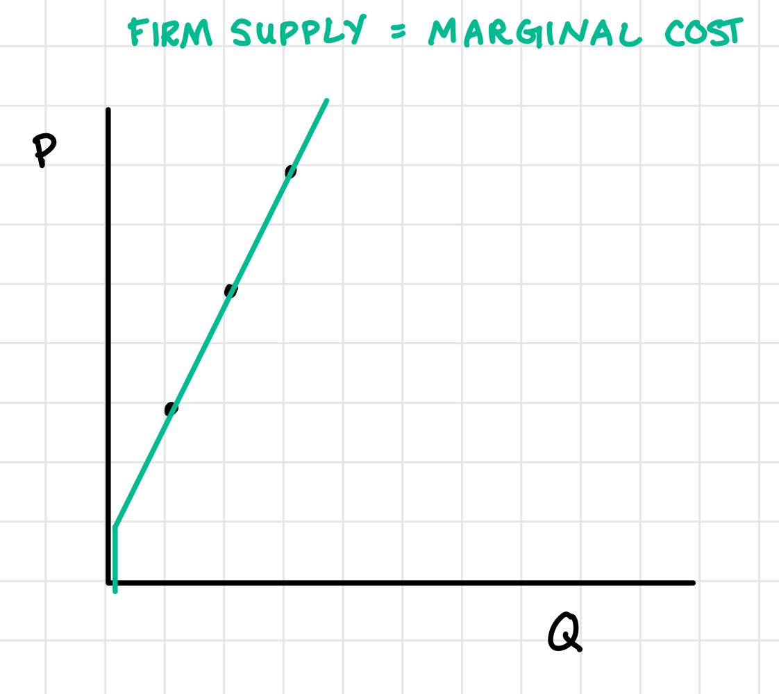
Let’s use a concrete example. Say your marginal cost function is \(MC = 2Q + 1\) and you face perfect competition.
If the market price for cakes is $5, you’ll solve: \(5 = 2Q + 1\), and bake \(Q = 2\) cakes.
If the market price rises to $7, you’ll produce more: \(7 = 2Q + 1\), and you’ll bake \(Q = 3\) cakes.
Note: in a perfectly competitive market, your marginal cost curve is your firm supply curve. And the market supply curve is the horizontal sum of firm supply curves, or firm marginal costs.

15.2 Long-Run Adjustment Processes in Perfect Competition
Constant-Cost Industries
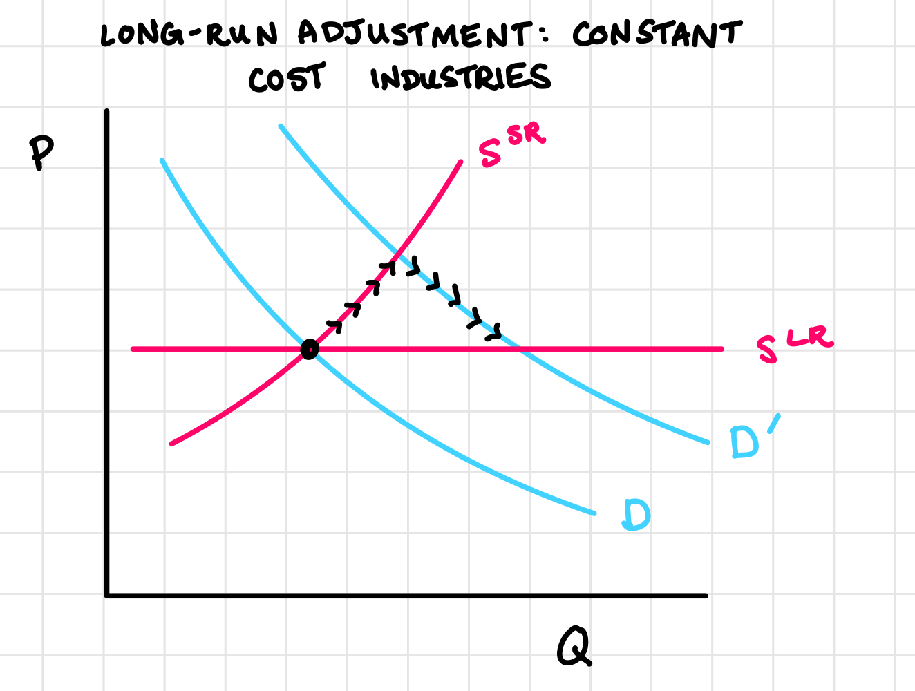
Consider the market for pencils. Whether suppliers produce a million pencils or a billion pencils, the cost to produce a pencil remains relatively stable. The prices of wood, graphite, and erasers are not significantly bid up when more pencils are produced.
In this “constant-cost” world, the long-run supply curve is flat (horizontal). No matter how many pencils are produced and sold, it always costs the same per unit.
If demand for pencils suddenly increases, in the short run, prices go up and existing firms increase the quantity they supply as much as they can, but their capabilities to do so are limited because some inputs are fixed, like their factory size.
The rise in prices give existing firms a boost in profits, which, in the long-run, incentivize existing firms to increase supply and it also incentivizes new firms to enter the market. Quantity supplied increases and prices fall back to where they started, because the long-run supply curve is horizontal.

The key insight here is that industries like the pencil industry can expand without significantly driving up its own costs. This allows for a smooth adjustment process where increased demand for pencils is met by increased supply without long-term price increases.
Increasing-Cost Industries
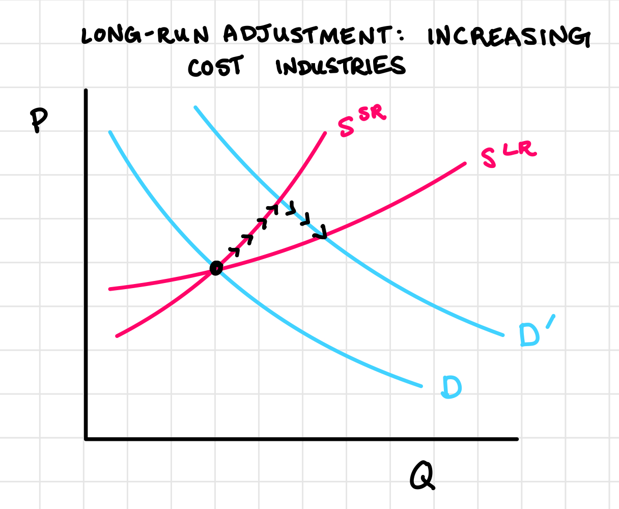
Now imagine an industry where expansion does drive up input prices. Maybe it’s an agricultural product like corn where using more land means using less fertile soil. Here, the long-run supply curve slopes upward. As the industry grows, costs increase.
To understand the dynamics in an increasing-cost industry, consider the example of consumer demand shifting from rice to corn. In the short run:
- Corn prices rise, rice prices fall.
- Corn producers earn profits and rice producers incur losses.
- But big changes in production are hard. Corn fields can’t appear overnight, and rice farmers can’t instantly switch crops.
In the Long Run:
- More farmers switch to corn, fewer grow rice.
- Corn supply increases more, dampening the price rise (but because of the upward sloping long-run supply curve, the price is still higher than before the shift in demand).
- Rice supply decreases more, softening the price fall (but the price is still lower than before the shift in demand).

This process shows the “invisible hand” in action. No central planner decided to shift resources from rice to corn. It happened through many individual decisions, all guided by prices and profit opportunities.
15.3 Classwork 15: Long-Run Equilibrium
Here’s some intuition for this classwork: in the short-run in a perfectly competitive market, it’s possible for firms to have positive economic profit (owners earn returns that _____ their opportunity cost). But in the long-run, those positive profits attract new entrants who expand industry _____, drive down prices, and erode existing firms’ _____. Market supply only stops increasing when economic profits hit zero.
Consider a perfectly competitive industry with the following characteristics:
Market demand: \(Q^d = 1000 - 20P\)
Market supply (short-run): \(Q^s = 5P\)
Find the short-run equilibrium price and quantity exchanged by setting \(Q^d = Q^s\). Use ggplot to graph the market demand and supply curves with P on the y-axis.
We know that the market is perfectly competitive, which means the representative firm is a price-taker. In the short-run, \(P^*\) is equal to (put your numeric answer from part a here), so in order to profit maximize, the representative firm will continue raising their supply \(q\) until their marginal cost is equal to the market price. Suppose the representative firm’s total cost is given by \(TC = 50 + 2q + 0.5q^2\), and calculate \(q\).
Calculate the representative firm’s profit.
Given the representative firm’s profit, should we expect that new firms will enter in the long-run? How will the market price change in response?
Continuing from question 2: assuming this is an increasing-cost industry with a long-run supply curve of \(Q = \frac{190}{3}P\):
Add this long-run supply curve to your ggplot from question 2. Why would an industry have increasing costs versus constant costs in the long-run?
In the long-run, what will happen to price and quantity in equilibrium?
Calculate the representative firm’s long-run profit.
A new example: suppose a representative firm’s long-run average cost is given by \(AC = 200 - 4 q + .05 q^2\).
If it operates in a perfectly competitive market, it will produce output \(q\) to minimize long-run average cost. Calculate that \(q\).
We learned the rule that when average cost is minimized, marginal cost is equal to average cost. Show that the rule holds given that the firm’s marginal cost is \(MC = 200 - 8Q + 0.15 Q^2\). Then give the intuition about why this rule holds (grading papers example).
If the price of the output good is _____ than the average cost, the firm will earn positive economic profit and new firms will start entering the market, driving \(P\) _____. Eventually, \(P\) will settle on the (competitive) firm’s minimum average cost, which is equal to their marginal cost.