1 Quarto: Markdown, LaTeX, and R

1.1 Typing up your Work

At the end of most weeks, you’ll need to type up your group’s answers to the classwork assignments and submit them online by 5pm. I require you to use Quarto for this because it’s the best tool for combining math proofs, written explanations, and R plots all in one place. Quarto makes everything look clean and professional—just like this workbook, which was created using Quarto. Submissions that are incorrectly or messily formatted won’t be accepted, so be sure to take advantage of what Quarto has to offer!

1.2 Setting up your Workspace

Grab a Computer

First things first, you should decide which computer you’d like to do your assignments on. It can be a Mac, Windows, or Linux machine: all are equally good. Laptops are better for this than desktops because you can bring them in to class. Please let me know ASAP if you don’t have a computer to use (chromebooks won’t work but there are workarounds I can discuss with you).

Download and Install R

Go here: https://cran.r-project.org/ and follow the instructions to download R for your Linux, Windows, or Mac. You should download the latest release.

Mac users: make sure you know whether you have an Apple silicon mac or an older intel-based mac and make sure that you download the correct version of R. If you’re not sure, hit the apple icon in your upper left hand corner and choose “About this Mac”. It might say something like Chip: Apple M1 (that’s apple silicon), or it might say something about Intel (that’s the intel mac).

If you’re using a mac, you’ll also need to install xquartz: https://www.xquartz.org/.

Install RStudio

Go here: https://posit.co/download/rstudio-desktop/ and click the blue button that says step 2: install RStudio Desktop.

Open RStudio and Install the Tidyverse

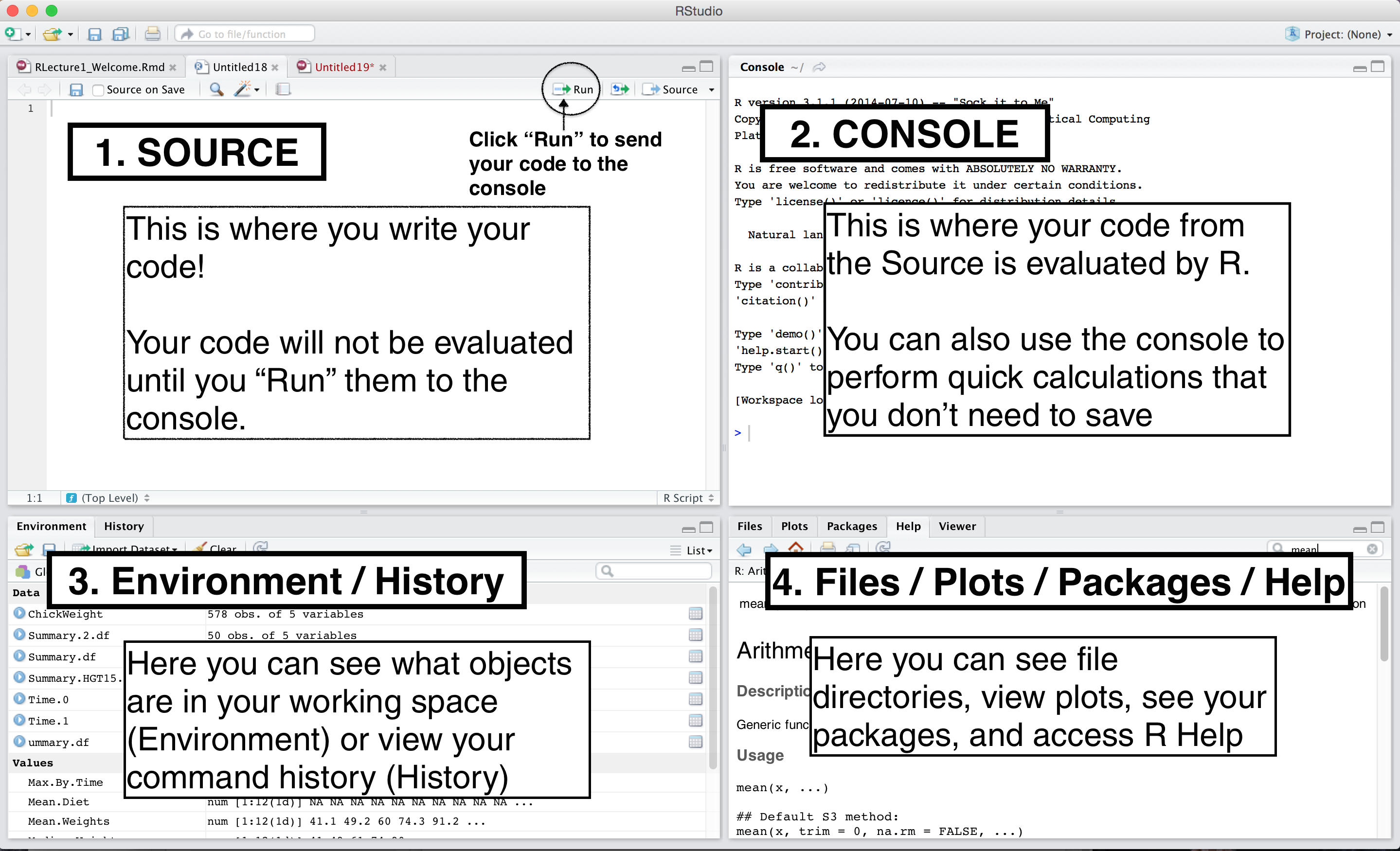
Open your new RStudio application. You should see 4 panels: source, console, environment/history, and files/plots/packages/help. For me, my console panel is below my source panel (unlike the image).

Copy-paste this line of code into your console and then hit return so that R runs it. This line of code installs the tidyverse, which is a collection of packages we’ll use to draw plots.

install.packages("tidyverse", dependencies = TRUE)

Now copy-paste these next lines of code into your console and hit return.

library(tidyverse)

ggplot() +
  stat_function(fun = function(x) 3 * x + 2, color = "red")

library(tidyverse) attaches the tidyverse package to your current session so you can use its functions (like ggplot()). Whenever you run library(tidyverse) in a new session, it will print a message detailing the packages and versions you’re attaching, along with conflicts. You can ignore that message.

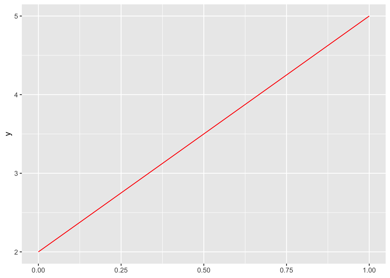
The ggplot lines of code draw the plot for the function $f(x) = 3x + 2$ in red.

If the plot of the line $f(x) = 3x + 2$ shows up in the lower right hand panel of RStudio, you’ve succeeded! If you’re not getting it or if you got stuck somewhere else, either come see me in office hours or try to see if a groupmate can help during class on Thursday.

1.3 Classwork 1: Recreate the Quarto Document

In this assignment, you will recreate a Quarto document that I’ve already compiled. You can only see the compiled HTML version, and your task is to reverse-engineer the quarto file by adding the necessary formatting, text, math, and code chunks in your own document. This exercise will help you become familiar with using Quarto, which you’ll need throughout the course.

Getting Started:

Open Rstudio and go to File > New File > Quarto Document.
Name the file Classwork 1 and enter you and your groupmates’ names under Author.
Keep the format at HTML and hit Create.

I’d recommend editing documents using the source editor versus the visual editor. You’ll want to periodically save your document (Command S on Mac, Ctrl S on Windows) and compile it to HTML (hit Render) to see your progress.

Hints

Text is formatted using markdown:

Use *text* or _text_ for italics.
Use **text** or __text__ for bold.
Use # for headings. The number of # symbols determines the heading level:
- # for Heading 1
- ## for Heading 2
- ### for Heading 3
Lists:
- For bullet points, use - or *.
- For numbered lists, use 1., 2., 3., etc.
Tables:
- Use pipes | to separate columns and hyphens - to create headers. For example:

    | This | is   | a     | table |
    |------|------|-------|-------|
    | with | some | words | in    |
    | it.  |      |       |       |

Math is formatted using LaTeX:

Math Mode
- Use $...$ for inline math.
- Use $$...$$ for display math (centered and in its own line).
Subscripts and superscripts
- Use _ for subscripts, e.g., x_i.
- Use ^ for superscripts, e.g., x^2.
Fractions
- Use \frac{numerator}{denominator}.
Special symbols:
- Use \sim for tilde, \partial for partial derivatives, \ln for natural logarithm.
Text inside math mode:
- Use \text{Words Here}.
Aligning Equations:
- Use the align environment to align equations. When you’re using the align environment, you don’t need to add any dollar signs to enter math mode. For example, use \begin{align}, \end{align}, and & to say where you want equations to align. The \\ indicates a line ending:

\begin{align}
y &= mx + b \\
z &= x^2 + y^2
\end{align}

Here’s how to add R code, especially to draw a plot:

Initialize an R Code Chunk:

    ```{r}

close it in another line with another three tics: ```
The first line of your code chunk should be: library(tidyverse). This command loads the tidyverse package into the session of the quarto document, which includes ggplot2, the package you’ll use to create the plot.
Then create a blank plot with the ggplot() function: ggplot()
Use the + operator to add layers to your plot. For example, to add a line representing the function $f(x) = 3x + 2$, use:

ggplot() +
  stat_function(fun = function(x) 3 * x + 2, color = "red")

Note that in R, multiplication uses the asterisk: *, addition uses +, subtraction uses -, division uses /, exponentiation uses ^, and parentheses can be used for grouping expressions:

(3 / 2) * 2 ^ 2

[1] 6