7 Consumer Behavior

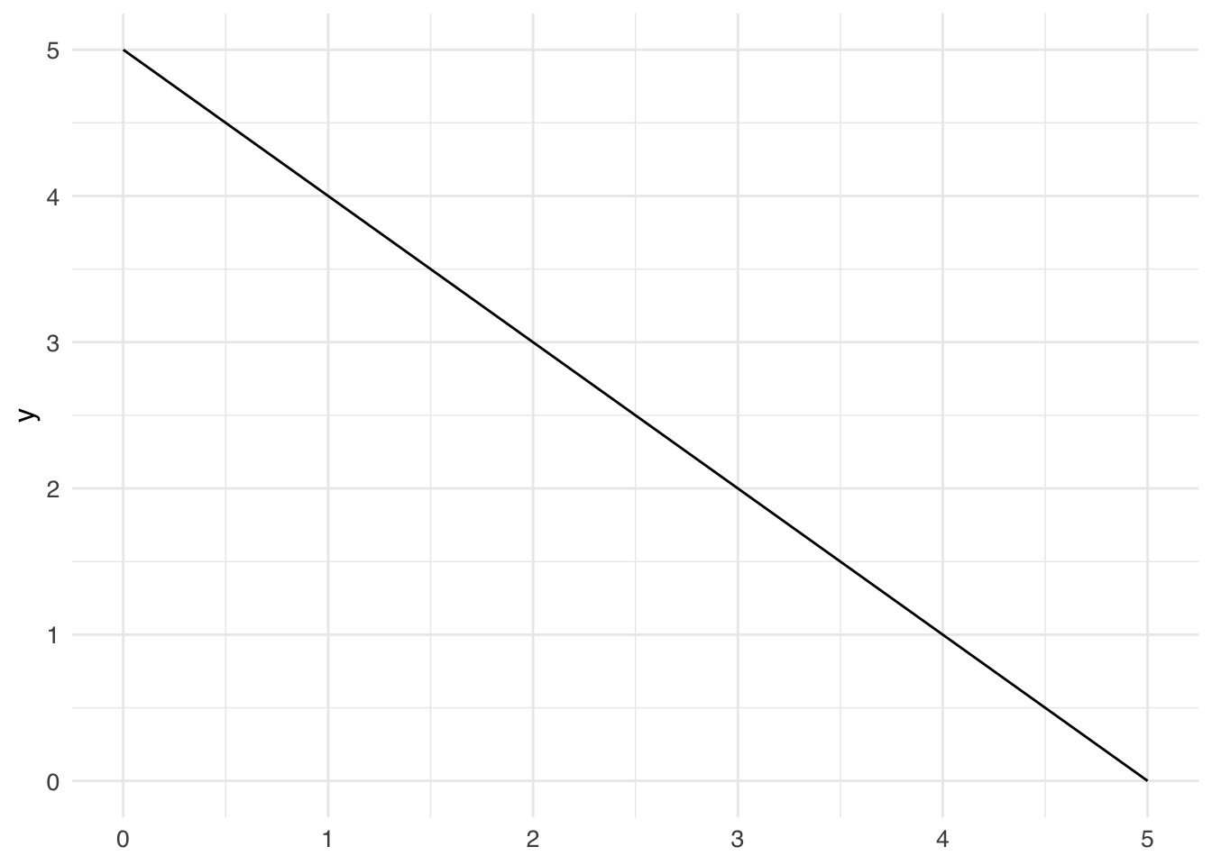
For more information on these topics, see Allen, Doherty, Weigelt, and Mansfield Chapter 3: Consumer Behavior and Rational Choice. Practice questions are from Marginal Revolution University.

When modeling consumer behavior, economists assume that consumers select the best bundle of goods they can afford. In this chapter, I’ll define that precisely as: consumers choose the bundle they most prefer from within their budget constraints.

7.1 Budget Constraints

Budget constraints are probably already very familiar to you. Consider this practice question to see how:

Practice Question: If your budget is $100, the price of a cup of coffee is $5, and the price of pizza is $10, can you afford to buy 10 cups of coffee and 6 pizzas?

Yes

You likely solved that practice question in the following way. For a bundle to be affordable, we need our total expenditure on pizza and coffee to be less than or equal to our budget:

\[p_{coffee}\cdot x_{coffee} + p_{pizza} \cdot x_{pizza} \leq m\]

Where $p_{coffee}$ refers to the price of coffee, $p_{pizza}$ refers to the price of pizza, $x_{coffee}$ refers to the number of coffees you’re trying to buy, $x_{pizza}$ refers to the number of pizzas you’re trying to buy, and $m$ refers to your budget.

If you consider bundles that exactly exhaust your budget (let $\leq$ become $=$) and then rearrange the equation above solving for $x_{pizza}$, you get a line in “slope-intercept” form:

\[\begin{align} p_{coffee}\cdot x_{coffee} + p_{pizza} \cdot x_{pizza} &= m\\ p_{pizza} \cdot x_{pizza} &= m - p_{coffee}\cdot x_{coffee}\\ x_{pizza} &= \frac{m}{p_{pizza}} - \frac{p_{coffee}}{p_{pizza}} x_{coffee}\\ \end{align}\]

This lets you see that the slope of the budget line is the price ratio $\frac{p_1}{p_2}$ and the y-intercept of the budget line is $\frac{m}{p_2}$.

A really easy way to draw a budget line is to figure out the y-intercept and the x-intercept and then connect those two points. The y-intercept is $\frac{m}{p_2}$ because the y-intercept is where you spend all your money on good 2. It says, you have $100 to spend, pizza costs $10 each, what’s the maximum number of pizzas can you buy? (the answer is 100/10 = 10).

The x-intercept can be found in a similar way: it’s $\frac{m}{p_1}$. The x-intercept is where you spend all your money on good 1. It says, you have $100 to spend, coffee costs $5 each, what’s the maximum number of coffees you can buy? It’s 100/5 = 20.

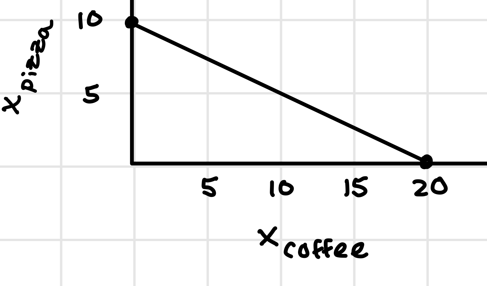
All bundles to the left of the budget line (or on the budget line) are affordable.

Budget line shows the market bundles that the consumer can purchase, given the consumer’s income and prevailing market prices.

Practice Question: Let the amount purchased of Good Y be drawn on the Y axis and let the amount purchased of Good X be drawn on the X axis. If the price of _________ is 2 and the price of __________ is 4, then the price ratio (or slope of the budget constraint) is 2.

Good X, Good Y

Good Y, Good X

7.2 Preferences

We’ll model consumer preferences using indifference curves:

Indifference Curve: contains points representing market bundles among which the consumer is indifferent.

Some important notes about indifference curves:

A consumer has many indifference curves. For simplicity, we’ll assume more is better: if bundle A has the same amount of one good and more of the other good compared to bundle B, the consumer prefers bundle A to bundle B. So bundles up and to the right are strictly preferred over bundles that are down and to the left.
Because more is better, for the consumer to be indifferent between bundle A and bundle B, bundle A must have a little more of one good, but a little less of another good compared to bundle B. Therefore, indifference curves must slope down and to the right.
Indifference curves can never cross. To see why:

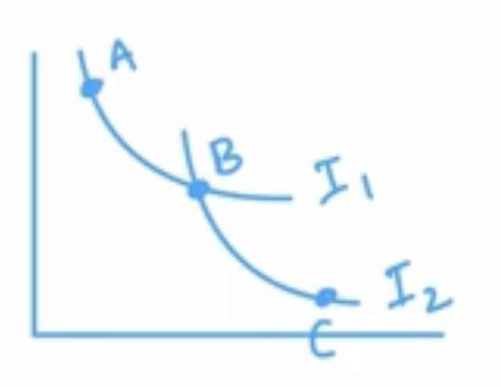
Suppose two indifference curves did cross: $I_1$ and $I_2$. Bundle B is the intersection. Because bundle A and bundle B are both on $I_1$, we know the consumer is indifferent between bundles A and B: $A \sim B$. Because bundle B and bundle C are both on $I_2$, we know $B \sim C$. By transitivity, we have that $A \sim C$, but this is a contradiction, because $I_1$ must contain all bundles X where $A \sim X$, but bundle C is not on $I_1$. Therefore, it’s impossible for two indifference curves to cross.

7.3 Marginal Rate of Substitution

The slope of the indifference curve (multiplied by -1) is the marginal rate of substitution. Recall that the slope of a line is $\frac{\text{rise}}{\text{run}}$.

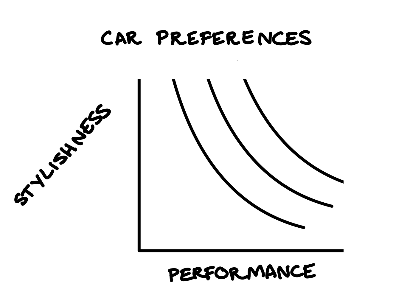
Marginal rate of substitution: the number of units of product Y that must be given up if the consumer, after receiving an extra unit of product X, is to maintain a constant level of satisfaction.

To illustrate: along their indifference curves, this car lover would be willing to give up lots of stylishness to get just a little more performance. A flatter indifference curve would indicate a preference for the opposite.

For the following question, assume Good X is measured on the x-axis and Good Y is measured on the y-axis.

Practice Question: A marginal rate of substitution of _____ means that, from the consumer’s point of view, 15 more units of Good Y is as good as 10 more units of Good X.

2/3

1.5

7.4 Choice

Utility indicates the level of enjoyment or preference attached by a consumer to a particular market bundle.

A utility function is a function that assigns a level of utility to any given bundle. Every bundle on a certain indifference curve has the same level of utility. So, indifference curves are level curves of a utility function.

We started this chapter saying that economists model consumer behavior as: consumers choose the bundle they most prefer from within their budget constraints. That is, they choose the bundle on the highest indifference curve that is still within their budget constraint.

I’ll plot the budget line $p_1 x_1 + p_2 x_2 = 5$ for the case where the price of both goods 1 and 2 are 1 and the consumer has an income of 5 to spend.

library(tidyverse)

ggplot() +
    stat_function(fun = function(x1) 5 - x1, color = "black") +
    xlim(0, 5)

Then I’ll add indifference curves of the utility function $u(x_1, x_2) = x_1 x_2$.

library(gganimate)

# Create data for the line and the point
point_data <- tibble(x = seq(5, 2.5, length.out = 100), y = 5 - seq(5, 2.5, length.out = 100))

p <- ggplot() +
    stat_function(fun = function(x1) 5 - x1, color = "black") +
    stat_function(fun = function(x1) 2/x1, color = "red") +
    stat_function(fun = function(x1) 4/x1, color = "orange") +
    stat_function(fun = function(x1) 6.25/x1, color = "gold1") +
    stat_function(fun = function(x1) 8/x1, color = "green") +
    stat_function(fun = function(x1) 10/x1, color = "blue") +
    xlim(0, 5) +
    ylim(0, 5) +
    geom_point(data = point_data, aes(x = x, y = y), color = "black", size = 3) +
    transition_reveal(along = -x)

animate(p)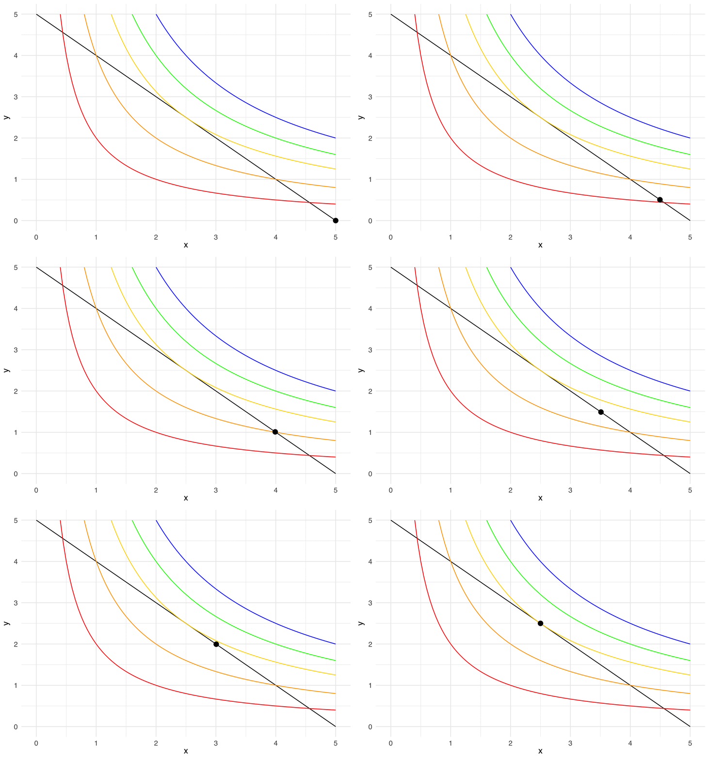

Let your eye follow the black dot along the budget line: along that line, the consumer exhausts their income on goods 1 and 2. The budget line crosses the red indifference curve ($u = 2$), so you know that the consumer can get more than a utility of 2. The budget line also crosses the orange indifference curve ($u = 4$), so you know that the consumer can get more than a utility of 4. Something interesting happens at the gold indifference curve ($u = 6.25$): the budget line doesn’t cross the gold indifference curve, the budget line is tangent to the gold indifference curve. The point of tangency represents the bundle that will earn the consumer the most utility ($u = 6.25$), while still being affordable.

As long as preferences are convex, indifference curves are smooth, and there is an interior solution, then the optimal choice $(x_1^*, x_2^*)$ is where the indifference curve is tangent to the budget line. At that point, the slope of the indifference curve (-1 times the MRS) is equal to the slope of the budget line ($-p_1/p_2$).

7.5 Classwork 7

Suppose you can either spend your money on pounds of food or on pieces of clothing. Sketch your budget line when a pound of food costs $5, a piece of clothing costs $50, and your income is $500. Use ggplot with stat_function when you’re typing this classwork up in quarto.
Select an option in order to fill in the blanks. For each part, explain your answer. You can refer to the budget line equation $x_2 = \frac{m}{p_2} - \frac{p_1}{p_2} x_1$.
- When you hold $p_1$ and $p_2$ constant and increase income $m$, your budget line (pivots to be steeper/pivots to be flatter/shifts out/shifts in).
- When you hold $p_1$ and $m$ constant and increase $p_2$, your budget line (pivots to be steeper/pivots to be flatter/shifts out/shifts in).
- When you hold $p_2$ and $m$ constant and increase $p_1$, your budget line (pivots to be steeper/pivots to be flatter/shifts out/shifts in).
Consider a consumer with indifference curves given by level curves of the utility function $u(x_1, x_2) = x_1 + 2 x_2$. What is the consumer’s marginal rate of substitution? Sketch some of the indifference curves (using ggplot with stat_function when you type this up).
Complete the sentences by making selections whenever there are parentheses: Continuing from part c, suppose the price ratio between the two goods is $\frac{p_1}{p_2} = 1$. Then the market values (good 1/good 2) more than the consumer does, and the consumer values (good 1/good 2) more than the market does. To maximize their utility, the consumer should buy zero units of (good 1/good 2) and spend their entire budget on (good 1/good 2). Add a couple examples of the budget lines with the price ratio of 1 to your plot in part c to show that your answers represent the point on the budget line reaching the highest possible indifference curve.