8 How Managers Can Strategically Influence Consumer Choices
For more information on these topics, see Allen, Doherty, Weigelt, and Mansfield Chapter 3: Consumer Behavior and Rational Choice.
8.1 Coupons
In the previous chapter, we discussed how microeconomic theory models consumer choices: consumers make decisions based on their budget constraint (which is determined by their income and the prices they face) and their indifference curves (which reflect their preferences).
Now, let’s consider how a manager might increase sales. Could they influence consumer preferences, incomes, or prices? While changing consumer incomes is difficult, the other two options are more feasible. Managers can run advertising campaigns to shift consumer preferences. Although they can’t directly change consumers’ incomes, they can impact consumer budget constraints by lowering their product’s price. For instance, consider a grocery store coupon that offers an $18 discount when you spend $180 in a single visit. How would this affect the consumer’s budget constraint?
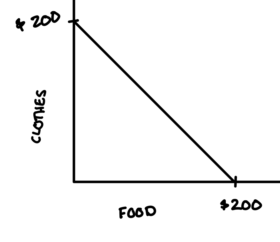
Before the coupon offer, here’s the budget constraint of a consumer with an income of $200, spending their income on either food or clothing. Let \(x_{food}\) refer to dollars spent on food and let \(x_{clothes}\) refer to dollars spent on clothes, so \(p_{food}\) and \(p_{clothes}\) are both equal to 1.

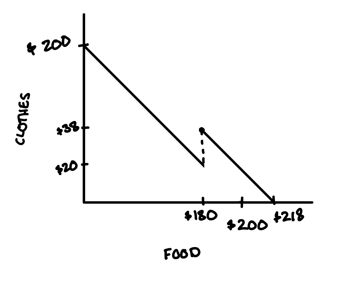
The coupon changes the consumer’s budget constraint. How? If you spend $180 or more on food, the grocery store takes off $18, allowing you to afford not $20 on clothes, but 20 + 18 = $38 on clothes. At maximum, you can afford not $200 on food, but $218. The coupon has the effect of shifting out your budget constraint at \(x_{food} \geq 180\), as if the grocery store has given you an extra $18 of income.

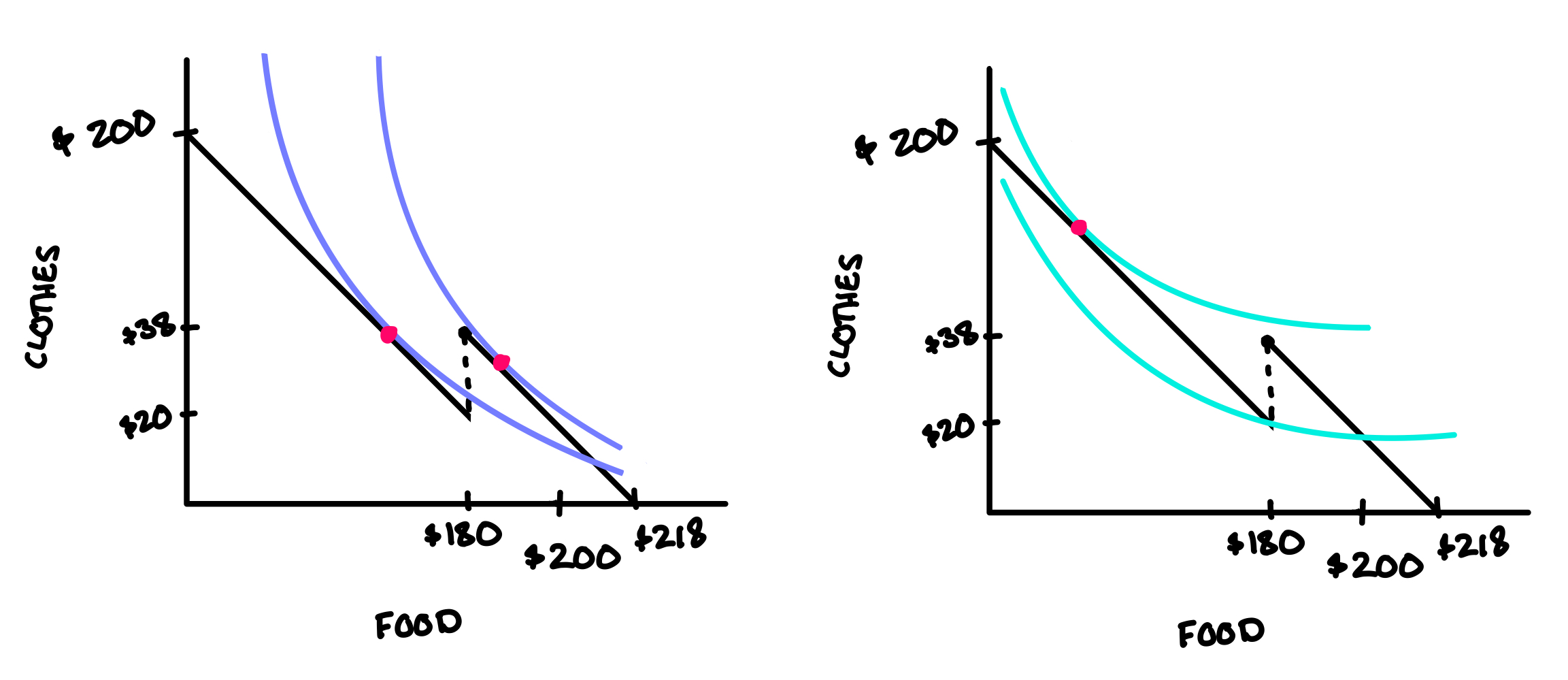
As you can imagine, such a coupon would be appealing to many consumers, but not all. If consumers have a strong enough preference for clothes over food (in terms of the marginal rate of substitution), they wouldn’t be willing to cut their spending on clothes in a sizeable enough way to even take advantage of the coupon.

Practice Question: In the figure above, which of the consumers would take advantage of the coupon for $18 back on a $180 grocery purchase?
Did the coupon increase the grocery store’s profit? Let’s consider three scenarios:
No one uses the coupon: In this case, the coupon policy has no impact on the grocery store’s profit, as there is no change in sales or revenue.
Most consumers typically spend $175: With the coupon, their spending increases to $180, but they pay only $162 due to the discount. Although more items are sold, the grocery store’s revenue decreases, making the coupon policy unprofitable.
Most consumers typically spend $140: With the coupon, their spending jumps to $180, while they pay just $162. This scenario boosts both the number of items sold and the store’s revenue, potentially leading to higher profits.
In summary, the coupon policy benefits the grocery store only when it significantly increases the spending of most consumers.
8.2 Deriving Individual Demand
So far, we know how to derive an individual’s choice given their income, the prices they face, and their utility function. Deriving their demand function takes it a step further: the demand function asks, for every given price of the good, how much will the consumer choose to buy?
An example: Let’s derive the demand curve for apples for a consumer with an income of $100. To find their optimal choices, we’ll let \(x_1\) refer to the number of apples they purchase and we’ll let \(x_2\) refer to the money they spend on all other things. Let the price of apples be $0.50. Suppose their utility function is given by \(u(x_1, x_2) = x_1^{\frac{1}{4}} x_2^{\frac{3}{4}}\). You might recognize this as a Cobb-Douglas utility function, which automatically tells you that the consumer will always choose to spend their income according to the exponents: the consumer will choose to allocate 1/4 of their income toward apples and 3/4 of their income toward other things. Let’s prove that this is the case:
- Note that this problem has only interior solutions because if the consumer spends all their money on just one good, they will buy zero of the other good and therefore get a utility of \(u = x_1 \times 0 = 0\). The Cobb-Douglas utility function means you have a strong preference toward mixtures of goods.
- We learned in the previous chapter that if preferences are convex and indifference curves are smooth, the interior solution is where the indifference curve is tangent to the budget line (they have the same slope). The slope of the budget line is \(-\frac{p_1}{p_2} = -\frac{.5}{1} = -\frac{1}{2}\). The slope of the indifference curve is the marginal rate of substitution, which is negative 1 times the partial derivative of u with respect to \(x_1\) divided by the partial derivative of u with respect to \(x_2\). : \(-\frac{\frac{\partial u(x_1, x_2)}{\partial x_1}}{\frac{\partial u(x_1, x_2)}{\partial x_2}}\). This comes from rearranging the total differential by letting \(du\) be zero (on an indifference curve, the change in utility is 0) and solving for \(\frac{\text{rise}}{\text{run}} = \frac{-dx_2}{dx_1}\).
- Setting the price ratio equal to the marginal rate of substituion, we get:
\[\begin{align} \frac{p_1}{p_2} &= \frac{\frac{\partial u(x_1, x_2)}{\partial x_1}}{\frac{\partial u(x_1, x_2)}{\partial x_2}}\\ \frac{1}{2} &= \frac{ \frac{1}{4} x_1^{-\frac{3}{4}} x_2^{\frac{3}{4}}}{ \frac{3}{4}x_2^{-\frac{1}{4}}x_1^{\frac{1}{4}}}\\ 3 &= \frac{2 x_2}{x_1}\\ 3x_1 &= 2x_2 \end{align}\]
- We have two unknowns: \(x_1\) and \(x_2\). To solve, we need two equations. Setting the price ratio equal to the marginal rate of substitution gave us our first one: \(3x_1 = 2x_2\). The second one comes from noticing that when the consumer exhausts their income, they maximize their utility. All their money should be spent on either apples or on other things, so the second equation is \(p_1 x_1 + p_2 x_2 = m\), or in this case, \(.5 x_1 + x_2 = 100\).
- Finally, we have two equations and two unknowns, so it’s straightforward to solve. I’ll use the fact that \(x_1 = \frac{2}{3} x_2\) from the first equation to plug in for \(x_1\) in the second equation:
\[\begin{align} .5 (\frac{2}{3}x_2) + x_2 &= 100\\ \frac{4}{3} x_2 &= 100\\ x_2 &= 75 \end{align}\]
- Now we can plug that back into any equation to find \(x_1\):
\[\begin{align} x_1 &= \frac{2}{3} x_2\\ x_1 &= \frac{2}{3} 75\\ x_1 &= 50 \end{align}\]
- So with the utility function of \(u(x_1, x_2) = x_1^{\frac{1}{4}} x_2^{\frac{3}{4}}\), where \(p_1 = .5\), \(p_2 = 1\), and \(m = 100\), the consumer buys 50 apples (which costs $25) and spends the other $75 elsewhere. Notice the Cobb-Douglas rule is verfied: the consumer spent 1/4 of their income on good 1 and 3/4 of their income on good 2.
Practice Question: Consider a consumer with the utility function \(u(x_1, x_2) = x_1^{.1} x_2^{.9}\). When they maximize their utility, how much of their income will they spend on good 1 and how much of their income will they spend on good 2?
- But we’re still not done: the demand function asks, for any given price of apples, how many apples will the consumer choose to buy? We’ll answer this question in Classwork 8.
8.3 Classwork 8
For parts a-c of this classwork, don’t worry about using ggplot to create your graphs. Hand-drawn graphs will be much easier for these exercises. Make sure everything is easy to read, and upload some sort of digital copy to Blackboard before the due date.
Imagine you have $4 to spend and you go to Dunkin Donuts. You can either spend your money on donuts at Dunkin or save it to spend later in the day at another store. Draw a budget constraint with donuts on the x-axis and money spent on other things on the y-axis. Let the price of “money spent on other things” be $1 (a dollar spent on other things costs you a dollar), and let the price of donuts be 50 cents each. Although the budget line is technically a step function because donuts are purchased in whole quantities, draw it as a straight line and add dots to represent the different discrete bundles that exhaust your $4 budget.
Now, suppose Dunkin Donuts offers a quantity discount: one donut costs 50 cents, a half dozen costs $2, and a dozen costs $3. Draw a new budget constraint, keeping in mind how much money you’ll have left after buying different amounts of donuts. For instance, how much money remains if you buy one donut? Two donuts? And so on.
Next, consider a consumer whose indifference curves reflect a preference for more donuts and more money left over. Given the quantity discount from part b, can you draw indifference curves where the consumer buys exactly 1 donut? What about exactly 4 donuts? Or 8 donuts? What are the quantities of donuts that such a consumer might choose to buy?
Now for a different question: continuing from where the workbook left off at the end of chapter 8, if a consumer’s utility function is \(u(x_1, x_2) = x_1^{\frac{1}{3}}x_2^{\frac{2}{3}}\), what type of utility function is this? If the consumer has $60 to spend, how much will they spend on good 1 and how much will they spend on good 2? Showing your work is not necessary.
Continuing from part d: let good 1 refer to pounds of food and let good 2 refer to money spent on everything else. If food costs $1 a pound, the consumer has an income of $60, and the consumer has the utility function \(u(x_1, x_2) = x_1^{\frac{1}{3}}x_2^{\frac{2}{3}}\), how much food will they choose to buy when they maximize their utility subject to their budget constraint? What if the price of food goes up to $2 a pound? What if the price of food goes down to just 50 cents a pound?
Continuing from part e: find the consumer’s demand function \(q(p)\): the number of pounds of food the consumer decides to purchase as a function of the price of food. Is the consumer’s demand function downward sloping? Use
stat_functionto sketch the consumer’s demand function using ggplot.