15 Omitted Variable Bias
Reading: Dougherty Chapter 6.1-6.2 (pages 261 - 272)
15.1 The Earnings-Education Question
The field of Education Economics is concerned with, more than anything else, this regression:
\[\text{Earnings}_i = \beta_0 + \beta_1 \text{Years of Education}_i + u_i\]
Take any dataset, around the world, throughout history, add as many other explanatory variables as you like (field, industry, gender, experience, parent’s education, etc) and you’ll find that the years someone spends in school seems to have an incredibly large and positive effect on their earnings down the road. And that makes sense: education should give you the skills and the new ways of thinking that ensure you’ll be successful in the real world. If it didn’t, what would be the point?
The thing is, the size of that \(\hat{\beta}_1\) is so large and positive that you have to wonder: if education is such a good investment, why do so many people drop out of high school? Why do so many people not go to college (when the cost of student loans is miniscule compared to the boost you seem to get to lifetime earnings)? Why do so many people drop out of college? As economists, we don’t usually like to chalk things up to irrational behavior. There has to be something else going on!
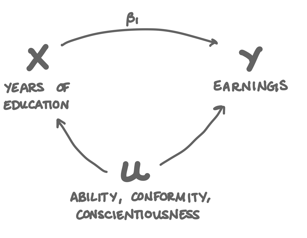
The answer is that there is omitted variable bias in that regression. There are variables that are really, really important in determining someone’s earnings, those variables are really hard to measure, and those variables are also highly correlated with how much education someone has received. They are: ability, conscientiousness, and conformity.
High ability people get more education because school is easy for them, and then they go on to have successful careers, but not necessarily because of their educations. Very conscientious people turn in better assignments both in school and at work. People who are conformists are more likely to stay in school and get along better in the workplace.
There’s no good way to measure ability, conscientiousness, and conformity, so when we have to leave them out of the earnings ~ education regression, because they’re correlated so strongly with both earnings and education, they confound the earnings-education relationship we’re trying to understand. What if it’s not because someone has so much education that they’re successful; what if it’s because they have a high ability, they’re very conscientious, or they’re a conformist? Only given observational data on people’s salaries and educations, we can never know which one it is.
When we have to omit ability, conscientiousness, or conformity from that earnings-education model, we can’t tell whether someone’s high earnings is because of their education, or because of their high ability, conscientiousness, or conformity. As a result, education always appears to be a much better investment than it probably actually is.
15.2 Another Example
Consider another example: \[\text{High School GPA}_i = \beta_0 + \beta_1 \text{Number of Friends of the Opposite Sex}_i + u_i\] Policymakers who are interested in whether same-sex schools are good for student performance might be interested in estimating this kind of model and getting an unbiased estimate for \(\beta_1\).
Exercise 1: If a variable that’s important to the data generating process for \(y\) is not included as an explanatory variable, then its affect is absorbed into \(u\). For example, in the earnings ~ education model, \(u\) absorbs ability, conscientiousness, and conformity because they help determine a person’s earnings. Which of these variables would be absorbed into \(u_i\) in the HS_GPA ~ opposite_sex_friends model directly above? Select all that apply.
a) Quality of study habits
b) Having strict parents
c) Number of friends of the same sex
d) Number of friends of the opposite sex
e) Mental and physical health
f) Test-taking skills
g) High School GPA
Exercise 2: A variable \(z\) that’s absorbed into \(u\) confounds the relationship between observed variables \(x\) and \(y\) if:
a) \(z\) affects \(x\)
b) \(z\) affects \(y\)
c) \(z\) affects \(x\) or \(z\) affects \(y\)
d) \(z\) affects \(x\) and \(z\) affects \(y\)
Exercise 3: Fill in the blank: Omitting “quality of study habits” would not confound the relationship between “number of opposite sex friends” and “high school GPA” because “quality of study habits” (does/does not) affect “number of opposite sex friends” while “quality of study habits” (does/does not) affect “high school GPA”.
a) does; does
b) does; does not
c) does not; does
d) does not; does not
Exercise 4: Fill in the blank: Omitting “strict parents” would confound the relationship between “number of opposite sex friends” and “high school GPA” because “strict parents” (does/does not) affect “number of opposite sex friends” while “strict parents” (does/does not) affect “high school GPA”.
a) does; does
b) does; does not
c) does not; does
d) does not; does not
Without a measure of how strict someone’s parents are, you wouldn’t be able to figure out whether the person’s high GPA was because they didn’t have a lot of friends of the opposite sex, or because they have strict parents who strongly encourage them to both get good grades and not make friends of the opposite sex.
15.3 Exogeneity
In this week’s classwork, I’ll explain how omitted variable bias comes down to a failure of the exogeneity assumption (\(E[u_i | X] = 0\)). To prepare for that, here’s a quick refresher on conditional expectations.
15.3.1 Conditional Expectations
The expectation of a random variable \(E[X]\) is its long-run average. If you roll a fair, six-sided die many many times, on average you’ll get the outcome of 3.5 because \(E[X] = \sum_i p_i x_i = \frac{1}{6}(1 + 2 + 3 + 4 + 5 + 6) = 3.5\).
The conditional expectation of a random variable \(X\) is its expectation conditioned on some other random variable \(Z\). For example the conditional expectation of a dice roll given an unrelated coin flip would be:
\[\begin{equation} E[\text{Dice Roll} \mid \text{Coin Flip}] = \begin{cases} 3.5, & \text{if heads} \\ 3.5, & \text{if tails} \end{cases} \end{equation}\]
Exercise 5: Evaluate this conditional expectation: \(E[\text{Dice Roll} \mid \text{the same dice roll is or is not greater than 3}]\)
a) 2 if the dice roll is not greater than 3 and 5 if the dice roll is greater than 3.
b) 3.5 if the dice roll is not greater than 3 and 3.5 if the dice roll is greater than 3.
c) 5 if the dice roll is not greater than 3 and 2 if the dice roll is greater than 3.
d) 3 if the dice roll is not greater than 3 and 3 if the dice roll is greater than 3.
If females are 63 inches on average and males are 69 inches on average, then the conditional expectation of height given sex is:
\[\begin{equation} E[\text{Height} \mid \text{Sex}] = \begin{cases} 63, & \text{if female} \\ 69, & \text{if male} \end{cases} \end{equation}\]
Exercise 6: Assuming the conditional expectation above is true, if a population is 100% female, what is \(E[Height]\) in that population?
a) 66 inches
b) 69 inches
c) 63 inches
d) 64.5 inches
Exercise 7: Assuming the conditional expectation above is true, if a population is 100% male, what is \(E[Height]\) in that population?
a) 66 inches
b) 69 inches
c) 63 inches
d) 64.5 inches
Exercise 8: Assuming the conditional expectation above is true, if a population is 50% male and 50% female, what is \(E[Height]\) in that population?
a) 66 inches
b) 69 inches
c) 63 inches
d) 64.5 inches
Exercise 9: Reflecting on the last couple questions, is a conditional expectation \(E[X | Z]\) equivalent to the unconditional expectation \(E[X]\) in the general case?
a) Yes, they are equivalent. \(E[X | Z]\) is always equal to \(E[X]\).
b) No, they are not equivalent. \(E[X | Z]\) will not always be equal to \(E[X]\).
Males and females both have average IQ’s of 100, so the conditional expectation of IQ given sex is:
Exercise 10: Assuming the conditional expectation above is true, if a population is 100% female, what is \(E[IQ]\) in that population?
a) 100
b) 120
c) 110
d) 80
Exercise 11: Assuming the conditional expectation above is true, if a population is 100% male, what is \(E[IQ]\) in that population?
a) 100
b) 120
c) 110
d) 80
Exercise 12: Assuming the conditional expectation above is true, if a population is 50% male and 50% female, what is \(E[IQ]\) in that population?
a) 100
b) 120
c) 110
d) 80
Exercise 13: Reflecting on the last couple questions, when is it true that the unconditional expectation of something is the same as the conditional expectation?
a) The conditional expectation will always be different from the unconditional expectation.
b) The conditional expectation will always be the same as the unconditional expectation.
c) When the conditional expectation is a constant, then the unconditional expectation will be that same constant.