Reading: If you want a little more information about the topics in this chapter, take a look at Dougherty Chapter 4.1 and Chapter 4.3.
When you’re reading papers in applied economics, you’ll often see models with transformations of variables (squared, interacted with other variables, logs of variables). This chapter and the next one offers some explanation about why you’ll see those things. All of these models can be estimated using OLS because they are either linear in parameters \(beta\), or they can be transformed into a model that is linear in parameters.
There are lots of instances where nonlinear relationships are more plausible than linear ones. Consider the students dataset again. I’ll coerce study_time and alcohol to be numeric.
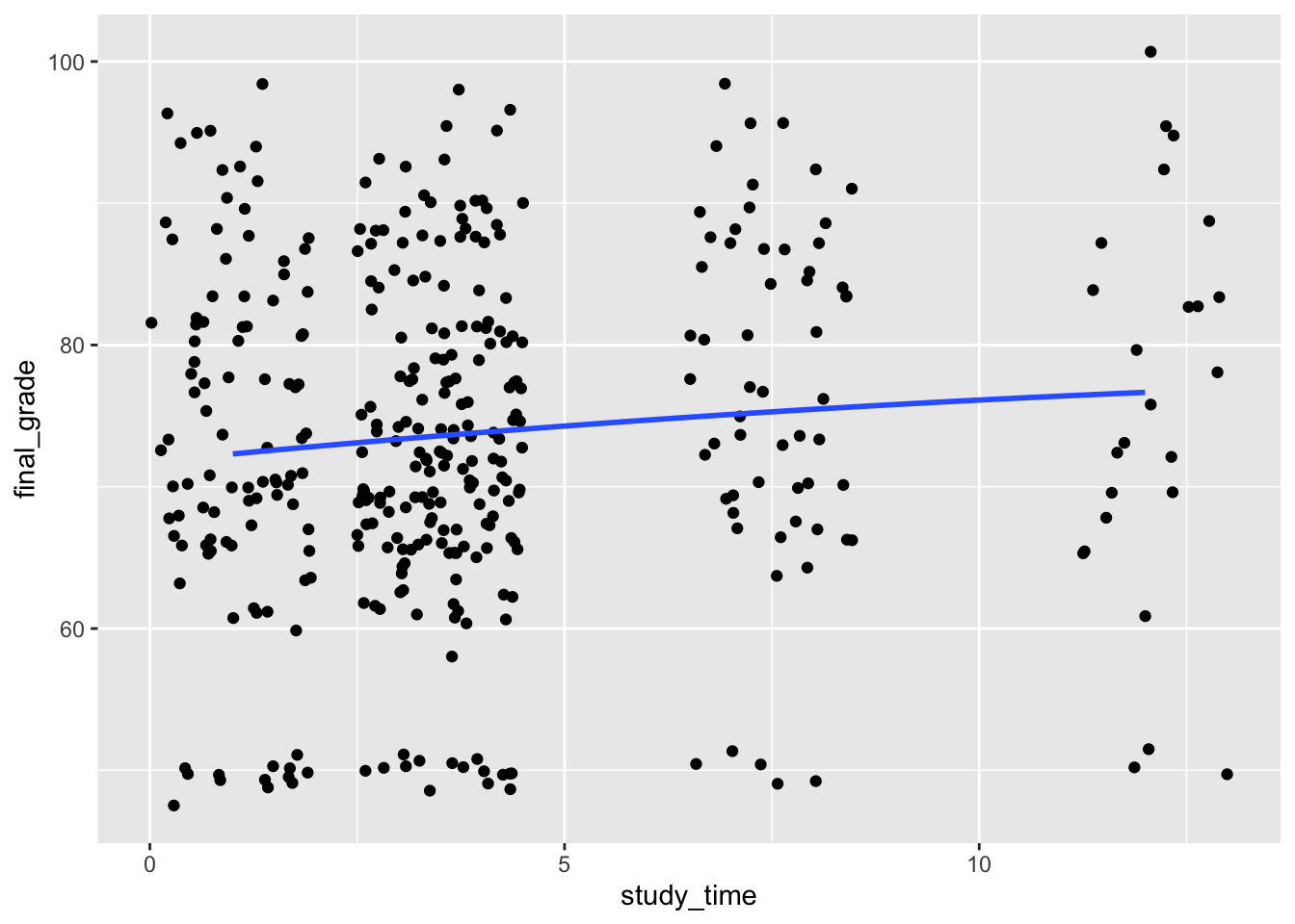
Fitting the model \(final\_grade = \beta_0 + \beta_1 study\_time + u\) gives us an estimate for \(\beta_1\) of 0.411 which is significant at the 0.10 level. The interpretation is that, for every extra hour per week a student spends studying, their final grade is expected to increase by 0.411 percentage points. But if someone studied for 100 hours per week, would they continue to see just as high returns per hour of studying? As an economist, you might be doubtful: something like studying would likely have diminishing marginal returns. And even with very limited data, that’s what seems to be going on:
students %>%ggplot(aes(x = study_time, y = final_grade)) +geom_jitter() +geom_smooth(method = nls, # nls stands for "nonlinear least squares"formula = y ~ a + b * x + c *I(x^2), # you can specify a model heremethod.args =list(start =c(a =1, b =1, c =1)), # you need to give the nls starting points for its search to find estimatesse = F # turn off standard error ribbons )
Grades improve with study time, but after a while, the improvement starts slowing down. You can model diminishing marginal returns by adding a squared term to your model like this:
students %>%lm(final_grade ~ study_time +I(study_time^2), data = .) %>% broom::tidy()
The capital I in the I(study_time^2) stands for “inhibit”. It “inhibits the evaluation” of study_time^2 so that lm understands that we want to add the square of the variable to the model as an explanatory variable.
The interpretation of this model: grades rise with study time, but that effect eventually wears off (although neither parameter is statistically significant). Going from 0 to 1 hour of studying is expected to increase your grade by .575 - .0138 = .5612 percentage points, but going from 10 to 11 hours is only expected to increase your grade by .575 * (11 - 10) - .0138 * (11^2 - 10^2) = .285 percentage points. In fact, the marginal contribution of studying is \(0.575 - 2 \times .0138 \times study\_time\).
Exercise 1: When should we expect that x^2 is perfectly correlated with x?
a) Always
b) Whenever x is nonnegative
c) Whenever x only takes on the values 0 and 1
d) Never
Exercise 2: Suppose we estimated these coefficients for this model: \(final\_grade = 75 + .62 study\_hours - .04 study\_hours^2\). What would be the expected increase to your final grade when you go from 0 to 1 hours of studying per week?
Exercise 3: Continuing from the previous question, what would be the expected increase to your final grade when you go from 10 to 11 hours of studying per week?
Exercise 4: Continuing again, what would we be estimating the marginal contribution of studying to be?
Consider a new model with study_time, failures, absences, and alcohol, all with squared terms included:
students %>%lm(final_grade ~ study_time +I(study_time^2) + failures +I(failures^2) + absences +I(absences^2) + alcohol +I(alcohol^2), data = .) %>% broom::tidy()
Exercise 5: How should we interpret the estimates on failures and I(failures^2)?
a) Each class you failed the previous year increases your expected grade by 10.4 percentage points, and if you failed many classes the previous year, that effect increases.
b) Each class you failed the previous year increases your expected grade by 10.4 percentage points, but if you failed many classes the previous year, that effect starts to wear off.
c) Each class you failed the previous year brings your expected grade down by 10.4 percentage points, and if you failed many classes the previous year, the effect is worse.
d) Each class you failed the previous year brings your expected grade down by 10.4 percentage points, but if you failed many classes the previous year, that effect starts to wear off.
Exercise 6: How should we interpret the estimates on absences and I(absences^2)?
a) Each absence you have decreases your expected grade by 0.331 percentage points, and with lots of absences, that effect gets worse.
b) Each absence you have increases your expected grade by 0.331 percentage points, but with lots of absences, that effect starts to wear off.
c) Each absence you have increases your expected grade by 0.331 percentage points, and with lots of absences, that effect continues to increase.
d) Each absence you have decreases your expected grade by 0.331 percentage points, but with lots of absences, that effect starts to wear off.