Reading: If you want a little more information about the topics in this chapter, take a look at Dougherty 1.6 and 2.1 (pages 107 - 114).
5.1 Chapter Preview
In this chapter I will define a regression’s \(R^2\), how to calculate it, and how to interpret it. Then I’ll discuss the differences between three data types, and I’ll introduce conditional expectations.
5.2\(R^2\)
When we do regression analysis, what we’re trying to do is to explain the data generating process for our dependent variable \(Y\). \(Y\) is sometimes low and sometimes high; to what extent could those variations in \(Y\) be explained by variations in \(X\), or is there just not a strong enough correlation?
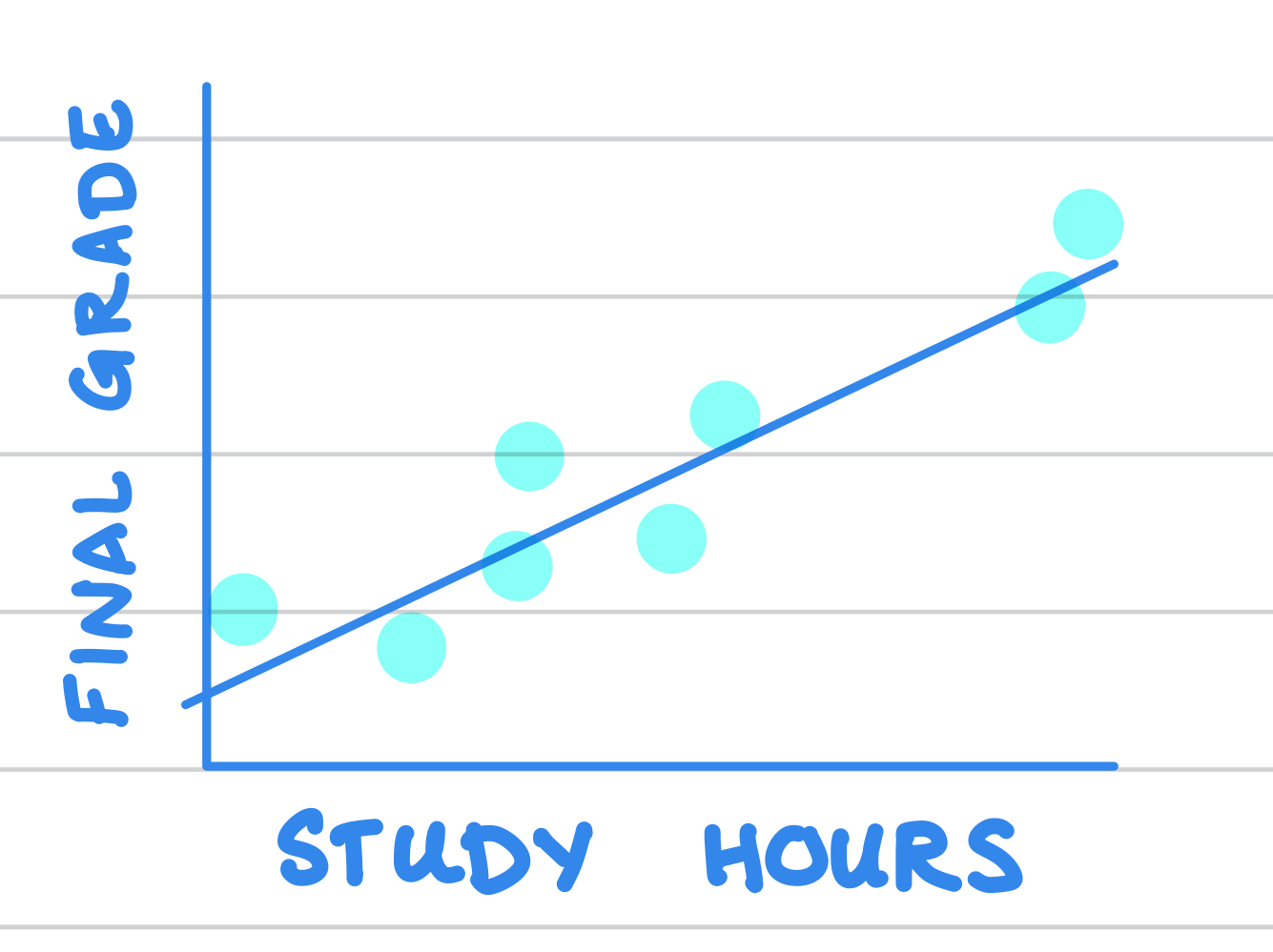
For example: take \(Y = final\_grade\) and \(X = study\_hours\), and consider the model \(final\_grade_i = \beta_0 + \beta_1 study\_hours_i + u_i\). By fitting this model, we’re trying to describe the data generating process for \(final\_grade\), especially how much a person’s \(final\_grade\) might be impacted by their \(study\_hours\). The unobservable term \(u_i\) contains the impact of any other variable on \(final\_grade\) other than study hours: the effectiveness of the student’s studying, attendance, knowledge of the subject matter, test-taking abilities, how well the instructor’s teaching style works for the student, the student’s physical and mental health, whether the student has anything else going on that could be a major distraction, etc!
If \(study\_hours\) is the dominant factor determining \(final\_grade\), we might end up with data that looks like Figure 5.1 (a). Assuming \(\hat{\beta}_0\) and \(\hat{\beta}_1\) are close to their true values, relatively small \(u_i\) will translate to relatively small residuals \(e_i\) and \(X\) and \(Y\) have a very strong linear correlation.
(a) Small residuals
(b) Large residuals
Figure 5.1: Two Scenarios for residuals \(e_i\)
But if \(study\_hours\) is just one important variable among many that explain \(final\_grade\), we might end up with data that looks like Figure 5.1 (b). Relatively large values for \(u_i\) translate to relatively large values for residuals \(e_i\) and, while \(X\) and \(Y\) are still correlated, the relationship isn’t as strong because \(X\) isn’t able to explain as much of the variation in \(Y\).
A regression’s \(R^2\) is the proportion of the variation in \(Y\) that can be explained by variation in \(X\) through the model: \(R^2 \equiv \frac{explained \ variation \ in \ Y}{total \ variation \ in \ Y} = \frac{\sum_i (\hat{y}_i - \bar{y})^2}{\sum_i (y_i - \bar{y})^2}\).
You can also show that \(R^2 = 1 - \frac{unexplained \ variation \ in \ Y}{total \ variation \ in \ Y} = 1 - \frac{\sum_i e_i^2}{\sum_i (y_i - \bar{y})^2}\) (proof in the Dougherty textbook). So we should expect that large residuals result in low values for \(R^2\). Figure 5.1 (b) should have a lower \(R^2\) than Figure 5.1 (a). The Dougherty textbook also shows that \(R^2\) is the square of the correlation between \(Y\) and fitted values \(\hat{Y}\) (hence the name \(R^2\)).
5.2.1 Numerical Example
In this numerical example, you will fill out the table below and use it to calculate the \(R^2\) from the regression \(y_i = \beta_0 + \beta_1 x_i + u_i\).
\(x_i\)
\(y_i\)
\(\hat{y_i}\)
\(e_i\)
1
5
2
10
3
9
Exercise 1: Calculate the model parameters \(\hat{\beta_0}\) and \(\hat{\beta_1}\). To do this, you can either use R (tibble() and lm()) or the formulas we derived: \(\hat{\beta_1} = \frac{\sum_i (x_i - \bar{x})y_i}{\sum_i (x_i - \bar{x})^2}\) and \(\hat{\beta_0} = \bar{y} - \hat{\beta_1} \bar{x}\).
Exercise 2: Use your calculations for \(\hat{\beta_0}\) and \(\hat{\beta_1}\) in the previous question to fill out the column for fitted values \(\hat{y_i}\). Recall that \(\hat{y_i} = \hat{\beta_0} + \hat{\beta_1}x_i\). You can either use that formula or the R function fitted.values().
Exercise 3: Now calculate the residuals \(e_i\). Use residuals() or the formula \(e_i = y_i - \hat{y_i}\).
Exercise 4: Finally, calculate the regression’s \(R^2\) and give an interpretation of what that statistic means.
A last word about \(R^2\): low values for a regression’s \(R^2\) doesn’t mean that the model is a failure. It just means that the model can only explain a small percentage of the total variation in the dependent variable. For instance, when the dependent variable is something like wages, economists usually expect their regressions to have an \(R^2\) around 0.20, and it would raise red flags to get a number a lot higher than that.
5.3 Data Types
There are 3 types of data that you’ll learn about studying econometrics:
Cross-sectional data
Time series data
Panel data
Cross-sectional data is the main focus of the Dougherty textbook, and it’s the only data type we’ll discuss in this class. In EC421, you’ll spend some time on time series and panel data.
What’s the difference? Cross-sectional data is data about many individuals at (around) the same time. Here, “individuals” might refer to people, or households, companies, cities, states, countries, etc. So a dataset describing student final grades and hours studying would be cross-sectional data:
# A tibble: 3 × 3
  name     study_time final_grade
  <chr>    <chr>            <dbl>
1 Chris    < 2H              69.4
2 Kourtney 2-5 H             89.7
3 Corey    < 2H              66.3
The name “cross-sectional” comes from the fact that the data is a cross-section of some population. It’s a snapshot in time of a sample of individuals.
Time series data, on the other hand, is about following one specific individual (or household, company, city, state, country) over time. So this dataset would be a time series if it reports quiz grades over the course of a term for one student:
And finally, panel data describes many individuals over many periods of time. For example, many students’ scores over the course of a term would be panel data:
If we have time series data, we can’t model it the same way we model cross-sectional data, and vice versa. The same thing goes with panel data. So all of this is to say: we’ll build models of exclusively cross-sectional data in this class, and you’ll study the other two types in EC421.
Exercise 5: Suppose you have some data on the daily closing price of a particular stock, every day for 3 months. Would that data be cross-sectional, time series, or panel data?
Exercise 6: Suppose you have a medical study’s data which tracks 30 patients’ health outcomes over time under different treatments. Would that data be cross-sectional, time series, or panel data?
Exercise 7: Suppose you have data from a market research survey that asked consumers about their preferences for different brands at one point in time. Would that data be cross-sectional, time series, or panel data?
5.4 Conditional Expectations
In the next chapter, I’ll show that the key assumption for \(\hat{\beta_1}\) to be an unbiased estimator of \(\beta_1\) (the true effect of \(X\) on \(Y\)) is that \(X\) is exogenous, which means that the conditional expectation of \(U\) given \(X\) is 0: \(E[U | X] = 0\). To understand what this is saying, we need a good firm grasp on conditional expectations of random variables.
The conditional expectation of a random variable is its expected value conditioned on other variables taking on certain values. An example can be useful:
Exercise 8: If there’s a population with 75% females and 25% males, what is \(E[height]\)?
Another conditional expectations example with an important result:
Exercise 9: Suppose that this is true: \[\begin{equation}
E[\text{{income}} | \text{{favorite color}}] =
\begin{cases}
30,000 & \text{{if favorite color = blue}} \\
30,000 & \text{{if favorite color = green}} \\
30,000 & \text{{if favorite color = pink}} \\
30,000 & \text{{if favorite color = purple}}
\end{cases}
\end{equation}\] What is \(E[income]\) in a population where 25% of people like blue the most, 25% of people like green, 25% of people like pink, and 25% of people like purple? Does \(E[income]\) depend on the proportions of types that exist in the population?
5.5 Summary
In this chapter, you learned:
A regression’s \(R^2\) measures how much of the total variation in \(Y\) is explained by the variation in \(X\).
There are 3 types of data you’ll come across in Econometrics: cross-sectional, time series, and panel data. You learned about how to distinguish between these.
A conditional expectation of a random variable is its expected value conditioned on other random variables taking on certain values. You learned that if the conditional expectation is a constant, then the unconditional expectation will be the same constant.