Reading: If you want a little more information about the topics in this chapter, take a look at Dougherty Chapter 4.
I’ll start this chapter reviewing a little about what what we’ve done so far, then what we did in Classwork 12, and finally I’ll end with a some new material on something called interactions, which concludes the material on using OLS to estimate nonlinear relationships.
13.1 Tidyverse Review
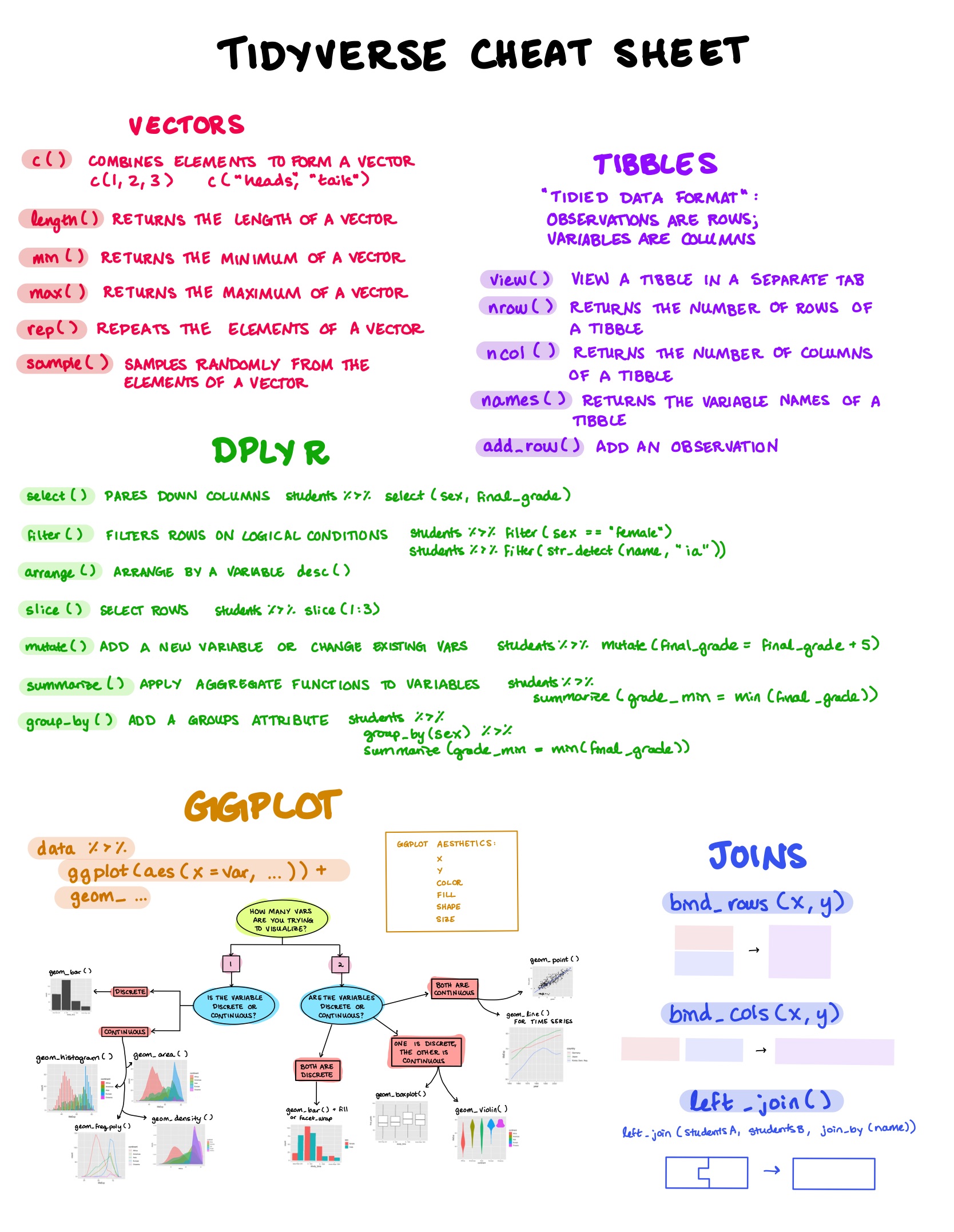
Here I’ve included a cheat sheet in order to remind you of some of the most important things we’ve learned about doing data analytics with the tidyverse. I think it’s pretty remarkable that, using a relatively small set of functions, you can do so much: take any dataset, answer any question about it, visualize it in any way you can imagine, and finally estimate a model of the data generating process of the variable of interest.
Broadly, an Econometrics course is all about getting you to think about data like an Economist. Economists like to make sure that our methodologies are backed by well-understood probability theory: we really don’t like to use methods that are “black boxes”. OLS is one of our favorite tools because so much is known about its theoretical foundations and it’s very versatile. So that’s exactly what we’ve been exploring in this class: the versatility of OLS and its theoretical foundations. In EC421, you’ll learn about the limitations OLS has and the different ways Economists try to circumnavigate those. OLS is definitely not the only method Economists use to do Econometrics, but it’s a very popular one.
13.2 Log Specifications
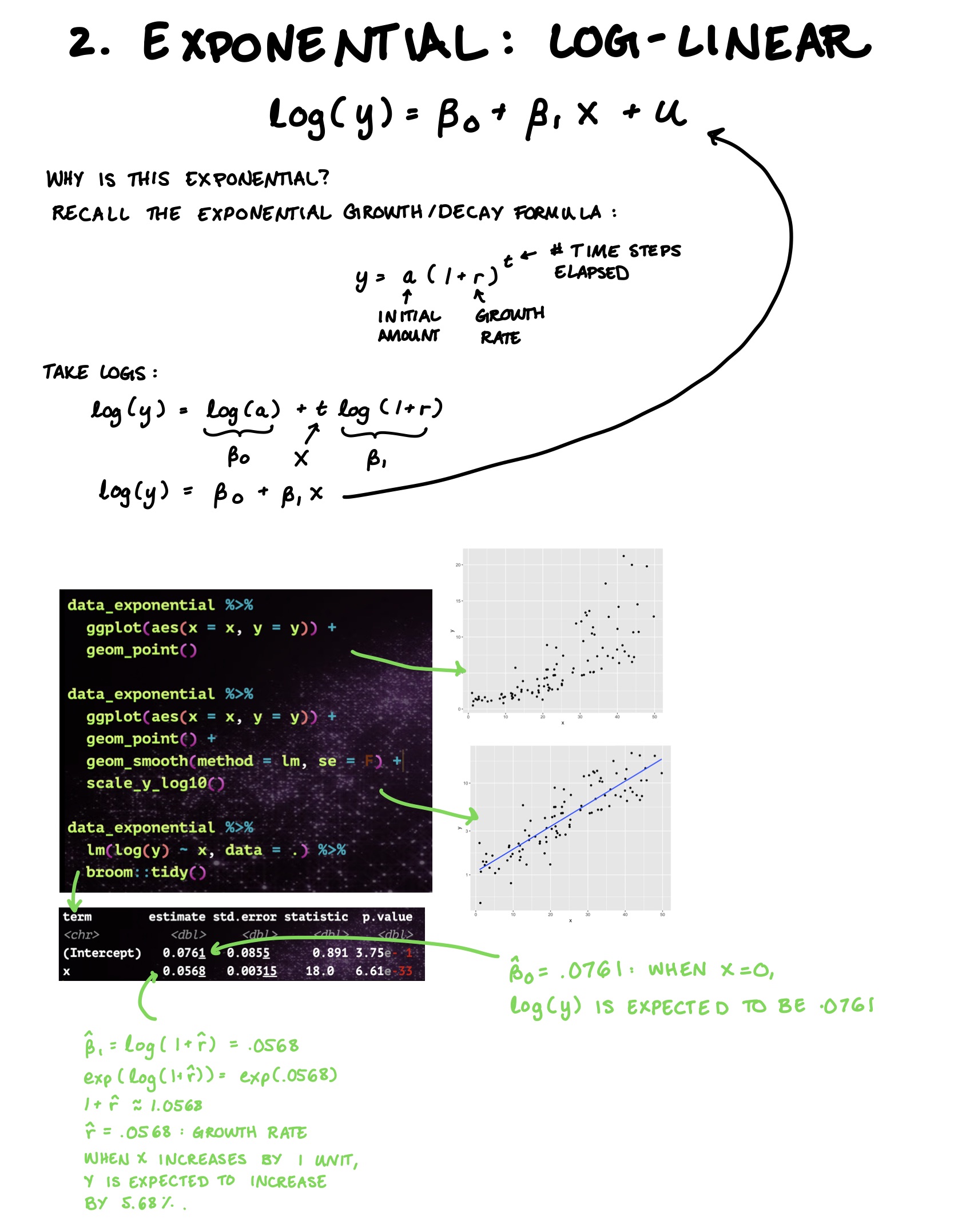
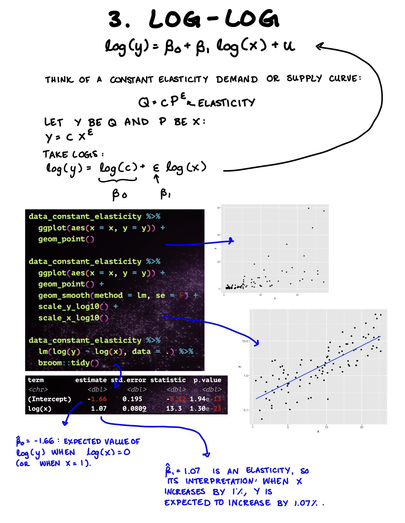
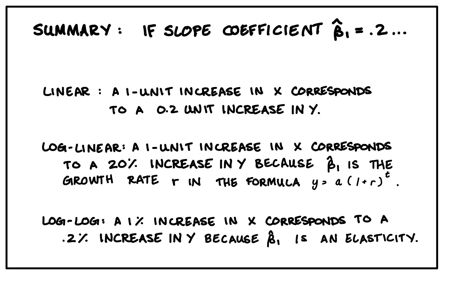
In Classwork 12, you learned a little about log-linear and log-log model specifications. Here’s a quick review.
13.3 Interactions
Now for the new material. An interaction is where we create a new explanatory variable that is equal to the product of two other explanatory variables. The two variables would usually appear in the model alone as well:
\[
y = \beta_0 + \beta_1 x_{1} + \beta_2 x_{2} + \beta_3 x_{1} x_{2} + u
\tag{13.1}\]
If you think that two variables, expecially when they act together, impacts \(y\), then an interaction term is appropriate to include.
Exercise 1: In Equation 13.1, if \(x_1\) increases by one unit, how much is \(y\) expected to increase by?
a) \(\beta_1\) units
b) \(\beta_1 + \beta_3\) units
c) \(\beta_1 + \beta_3 x_2\) units
d) \(\beta_1 + \beta_3 x_1 x_2\) units
As I explain in the video below, when one of the two variables in an interaction term is binary (takes only the values 0 and 1), then an interaction allows the slope between the two groups to differ. Disregard the prompting to launch the video from your course.
For the questions below, suppose you estimated this model:
Exercise 2: In Equation 13.2, how much would you predict a 6 foot male weighs?
a) 160
b) 170
c) 180
d) 190
Exercise 3: In Equation 13.2, how much would you predict a 6 foot female weighs?
a) 150
b) 160
c) 170
d) 180
Exercise 4: In Equation 13.2, what is the estimated impact of a one-unit (one foot) increase in height for a male person?
a) Increase of 20 lbs
b) Increase of 30 lbs
c) Increase of 40 lbs
d) Increase of 50 lbs
Exercise 5: In Equation 13.2, what is the estimated impact of a one-unit (one foot) increase in height for a female person?
a) Increase of 20 lbs
b) Increase of 30 lbs
c) Increase of 40 lbs
d) Increase of 50 lbs
Exercise 6: In Equation 13.2, which group has the steeper slope when it comes to how height (x) impacts weight (y)?
a) Males have a steeper slope.
b) Females have a steeper slope.
In R, you can estimate models with interactions using this symbol :
library(tidyverse)students <-read_csv("https://raw.githubusercontent.com/cobriant/students_dataset/main/students.csv")students %>%lm(final_grade ~ sex + failures + sex:failures, data = .) %>% broom::tidy()
13.4 Ramsey RESET (Test for Functional Misspecification)
Suppose you’re fitting a model that’s linear in variables:
\[y = \beta_0 + \beta_1 x + \beta_2 z + u\]
But visualizations point to the possible existance of nonlinear relationships in the model. You’re wondering if you need to include squared or interaction terms as explanatory variables, too. It turns out there’s a test for this, and it’s called the Ramsey RESET (Regression Equation Specification Error Test). Here’s how it works:
Step 1: get the fitted values from the model that’s linear in variables. Call this yhat.
Recognize that since \(\hat{y} = \hat{\beta}_0 + \sum_j \hat{\beta}_j x_j\), it’s true that \(\hat{y}^2 = (\hat{\beta}_0 + \sum_j \hat{\beta}_j x_j)^2\), which includes all possible squared terms and interactions.
Step 2: Run the same regression you did in step 1, but now with one more explanatory variable, the square of yhat: y ~ x + z + ... + I(yhat^2). A t-test on the coefficient for the yhat^2 term will indicate whether a squared or interaction term belongs in the model.
Exercise 7: What is the implication if the Ramsey RESET test is significant?
a) The model is perfectly specified.
b) There is no need to include squared or interaction terms.
c) The model may have an incorrect functional form.
d) The model’s assumptions are all met.