10 Multiple Regression
Reading: Dougherty Chapter 3 (pages 156 - 196)
10.1 A Model with 2 Explanatory Variables
Up until now, we’ve been working with the simple regression model where there is one explanatory variable and one dependent variable, like this:
\[\text{final\_grade} = \beta_0 + \beta_1 \text{study\_hours} + u\]
Multiple regression, on the other hand, lets us add as many other explanatory variables as we wish, like this:
\[\text{final\_grade} = \beta_0 + \beta_1 \ \text{study\_hours} + \beta_2 \ \text{absences} + \beta_3 \ \text{alcohol} + \beta_4 \ \text{romantic} + u\]
In the multiple regression model, parameters \(\beta\) have the very useful interpretation of the impact of changes in just one variable, holding others constant.
10.2 Example
If we think that a person’s final grade is determined solely by the number of hours they spend studying, then we should use the simple regression model:
\[\text{final\_grade} = \beta_0 + \beta_1 \text{study\_hours} + u\]
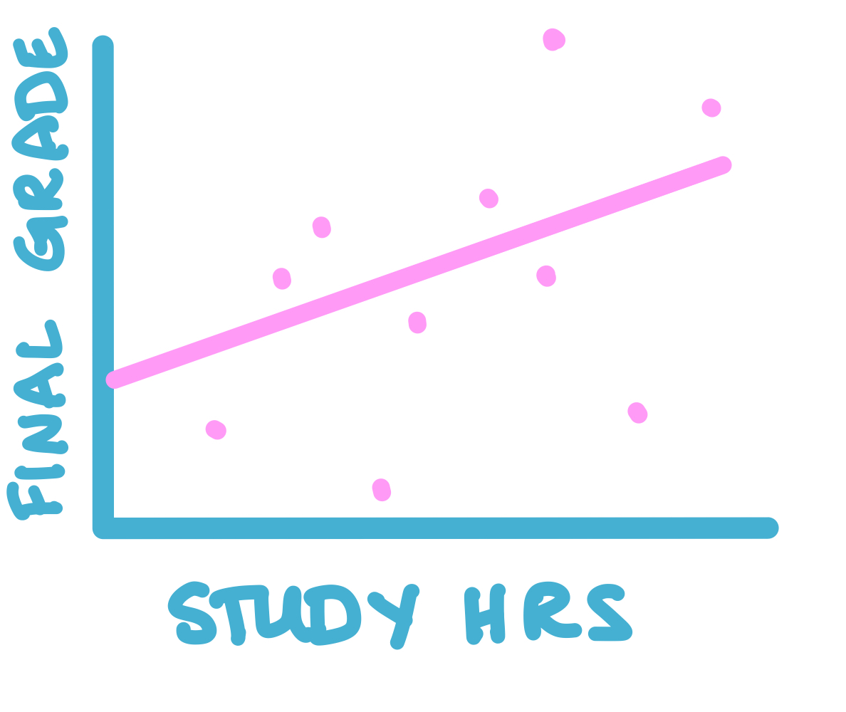
As you’ve already learned, the fitted values in the simple regression model tell you the predicted final grade for someone who has studied any given number of hours. So for example, you can use the fitted values to see the final grade that’s expected for someone who studies zero hours, and the final grade that’s expected for someone who studies for 30 hours.
Instead of a line, the multiple regression model (with 2 explanatory variables) can be visualized as a tilted plane in 3-dimensional space:
\[\text{final\_grade} = \beta_0 + \beta_1 \ \text{study\_hours} + \beta_2 \ \text{absences} + u\]
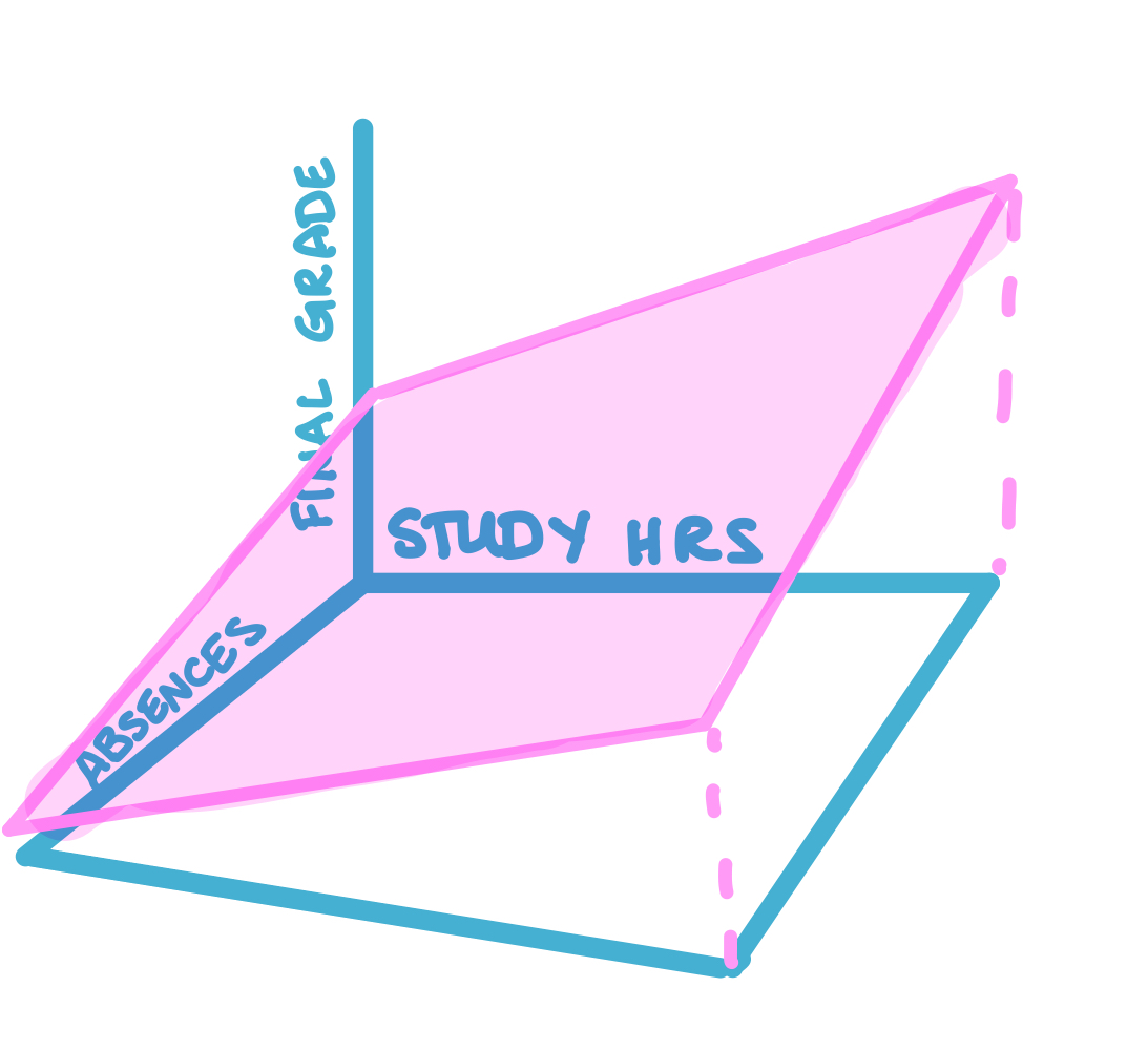
The fitted values in this multiple regression model would tell you the predicted final grade for someone who has studied a given number of hours and has a given number of absences. So for example, you can use the fitted values from a multiple regression model to find the final grade that’s expected for someone who studies 12 hours and has 2 absences.
Example: Suppose we take data on people’s final grades, their study hours, and the number of absences they have, we run the regression lm(final_grade ~ study_hours + absences), and we get these estimates: \(\text{final\_grade} = 73 + 2 \ \text{study\_hours} - 0.2 \ \text{absences} + u\). Then if someone studies zero hours and they have zero absences, their predicted final grade is \(\hat{\beta_0} = 73\).
Continue assuming that we’re working with these estimates for exercises 1-3: \(\text{final\_grade} = 73 + 2 \ \text{study\_hours} - 0.2 \ \text{absences} + u\)
Exercise 1: If someone studies 10 hours and has zero absences, what is their predicted final grade? What about someone who studies 0 hours and has 10 absences? What about someone who studies 10 hours and has 10 absences?
Exercise 2: Holding constant a person’s number of absences, what is the impact of an extra hour of studying on their predicted final grade?
Exercise 3: Holding constant a person’s study hours, what is the impact of an extra absence on their predicted final grade?
\(\hat{\beta_1}\) and \(\hat{\beta_2}\) are interpreted as the “pure effect” of only \(x_1\) or \(x_2\), which means that even though \(x_1\) and \(x_2\) may be correlated, using multiple regression accounts for this correlation and \(\hat{\beta_1}\) estimates the impact on \(y\) of a change to \(x_1\) alone. This can be justified in two ways: 1) showing \(\hat{\beta_1}\) is unbiased (we’ll skip this because it just comes down to exogeneity, just like in the simple regression context), and 2) exploring the Frisch-Waugh-Lovell theorem (we’ll do this in a classwork coming up soon).
10.3 Formulas for Multiple Regression with 2 Explanatory Variables
10.3.1 Estimates of Model Parameters
The derivation of formulas for \(\hat{\beta}\) follow the same pattern as the simple regression case. In a multiple regression model with two explanatory variables, you’ll get that:
\[\hat{\beta_0} = \bar{y} - \hat{\beta_1} \bar{x_1} - \hat{\beta_2} \bar{x_2}\]
Which you can compare to the simple regression formula: \(\hat{\beta_0} = \bar{y} - \hat{\beta_1} \bar{x_1}\).
And you’ll also get that:
\[\hat{\beta_1} = \frac{\sum x_1 y - \bar{x_1} \bar{y} n - \hat{\beta_2} (\sum x_1 x_2 - \bar{x_1} \bar{x_2}n)}{\sum x_1^2 - n \bar{x_1}^2}\]
Which you can compare to the simple regression formula: \(\hat{\beta_1} = \frac{\sum x y - \bar{x} \bar{y} n}{\sum x^2 - n \bar{x}^2}\).
10.3.2 Standard Errors
The variance of \(\hat{\beta_1}\) is:
\[\sigma^2_{\hat{\beta_1}} = \frac{\sigma^2_u}{\sum (x_1 - \bar{x_1})^2} \times \frac{1}{1 - \rho^2_{x_1 x_2}}\]
Where \(\rho_{x_1 x_2}\) is the correlation between variables \(x_1\) and \(x_2\). Recall that correlation is always between -1 and 1, so the square of a correlation is always between 0 and 1. Also recall that if two variables are not correlated, their correlation will be 0. Letting the mean squared deviation of \(x_1\) be \(MSD(x_1) = \frac{1}{n}\sum (x_1 - \bar{x})^2\),
\[\sigma^2_{\hat{\beta_1}} = \frac{\sigma^2_u}{n MSD(x_1)} \times \frac{1}{1 - \rho^2_{x_1 x_2}}\]
And you can derive the standard errors for the multiple regression model parameters by estimating this value using residuals \(e\) and taking the square root.
Example: Just like in the simple regression case, the formula for \(\sigma^2_{\hat{\beta_1}}\) shows us that multiple regression standard errors decrease as the sample size \(n\) increases because \(n\) is in the denominator. So multiple regression parameters are estimated more precisely with a large sample size.
Exercise 4: Is the multiple regression parameter \(\beta_1\) estimated more or less precisely when \(x_1\) is more spread out?
Exercise 5: Is the multiple regression parameter \(\beta_1\) estimated more or less precisely when u has a larger variance?
Exercise 6: Is the multiple regression parameter \(\beta_1\) estimated more or less precisely when \(x_1\) and \(x_2\) are highly corelated?
We’ll continue to explore the intuition behind the answer to exercise 6 in the next two classworks. When two or more explanatory variables are highly correlated, you have what’s called multicollinearity.