A dummy variable (also known as an indicator variable) is a binary variable that takes a value of 0 or 1. Dummy variables are used to encode categorical features. For example, you’d use a dummy variable for sex where sex might equal 0 for females and 1 for males. In this chapter, you’ll also learn how to use a set of dummy variables to encode categorical features which take on more than just two values.
14.2 Dummy Variable for 2 Categories
Creating a dummy variable to represent categorical data where there are only two groups is simple. Take, for instance, the variable sex in the students dataset:
# A tibble: 374 × 2
   sex    female
   <chr>   <dbl>
 1 female      1
 2 female      1
 3 female      1
 4 female      1
 5 male        0
 6 female      1
 7 female      1
 8 female      1
 9 male        0
10 male        0
# ℹ 364 more rows
I can use mutate to take sex and make a variable female which takes a 1 if the person is female and takes a 0 otherwise. Then I can use female in a regression:
students %>%mutate(female =if_else(sex =="female", 1, 0)) %>%lm(final_grade ~ female, data = .) %>% broom::tidy()
For a dummy variable, the reference category is the category that is left out of the regression, or in other words, it has a value of zero for every dummy. In the example above, the dummy variable is for the “female” category of sex, and the reference category is “male”.
Exercise 1: To interpret the regression output above, we’d say that:
a) On average, girls score 2.52 points lower than boys at math, but that is not significant at the .05 level.
b) On average, girls score 2.52 points lower than boys at math, and that is significant at the .05 level.
c) On average, boys score 2.52 points lower than girls at math, but that is not significant at the .05 level.
d) On average, boys score 2.52 points lower than girls at math, and that is significant at the .05 level.
That mutate step is actually redundant because lm will automatically coerce sex to be a dummy variable automatically:
students %>%lm(final_grade ~ sex, data = .) %>% broom::tidy()
Exercise 2: In the regression directly above, notice we estimate 2.52 instead of -2.52 for \(\hat{\beta}_1\). Which categories has lm chosen to be the reference category and the dummy variable?
a) The reference category is now male and the dummy variable is now female.
b) The reference category is now female and the dummy variable is now male.
14.3 Dummy Variable Trap
Why do we need to have a reference category and a dummy variable? Why can’t we just have dummy variables for both male and female? Notice lm gives us NAs when I try to do this:
students %>%mutate(male =if_else(sex =="male", 1, 0),female =if_else(sex =="female", 1, 0) ) %>%lm(final_grade ~ male + female, data = .) %>% broom::tidy()
# A tibble: 3 × 5
  term        estimate std.error statistic    p.value
  <chr>          <dbl>     <dbl>     <dbl>      <dbl>
1 (Intercept)    72.5      0.879     82.5   4.03e-241
2 male            2.52     1.24       2.03  4.34e-  2
3 female         NA       NA         NA    NA
Exercise 3: You need to leave one category out of a regression (you need to have a reference category) because if you don’t, one variable will be a perfect linear function of the other variables and you’ll get perfect multicollinearity. This is what’s known as the dummy variable trap. To see this, note that:
a) \(female = 1 + male\)
b) \(female = -1 + male\)
c) \(female = -1 - male\)
d) \(female = 1 - male\)
14.4 More than Two Categories
Consider a variable with more than two categories, like study_time. It can take on four different values: less than 2H, 2 - 5H, 5 - 10H, or more than 10H.
students %>%select(study_time)
# A tibble: 374 × 1
   study_time
   <chr>
 1 less than 2H
 2 less than 2H
 3 5 - 10H
 4 more than 10H
 5 2 - 5H
 6 2 - 5H
 7 2 - 5H
 8 2 - 5H
 9 2 - 5H
10 less than 2H
# ℹ 364 more rows
The way to approach this situation is to pick a reference category (less than 2H is a natural base category here), and then we’ll define a set of three dummy variables for the three other categories. Then there will be three explanatory variables:
To interpret the regression output above, realize that everything is in reference to the reference category:
Studying 2-5H instead of less than 2H provides a 0.127 point boost to final scores on average, but that estimate is not statistically significant at the .05 level.
Studying 5-10H instead of less than 2H provides a 3.87 point boost to final scores on average, and that estimate is statistically significant at the .10 level (although not at the .05 level).
Exercise 4: Interpret the estimate for the coefficient for study_veryhigh in the regression above.
a) Studying more than 10H instead of 5-10H provides a 2.86 point boost to final scores on average, but that estimate is not statistically significant at the .05 level.
b) Studying more than 10H instead of less than 2H provides a 2.86 point boost to final scores on average, but that estimate is not statistically significant at the .05 level.
c) Studying more than 10H instead of 5-10H provides a 2.86 point boost to final scores on average, and that estimate is statistically significant at the .05 level.
d) Studying more than 10H instead of less than 2H provides a 2.86 point boost to final scores on average, and that estimate is statistically significant at the .05 level.
Once again, using mutate to create dummies by hand is not necessary because lm does it automatically, even when the variable takes on more than two values:
students %>%lm(final_grade ~ study_time, data = .) %>% broom::tidy()
The issue here is that lm may not always automatically choose natural reference categories.
Exercise 5: In the regression above, which category has lm chosen to be the reference category?
a) Less than 2H
b) 2 - 5H
c) 5 - 10H
d) More than 10H
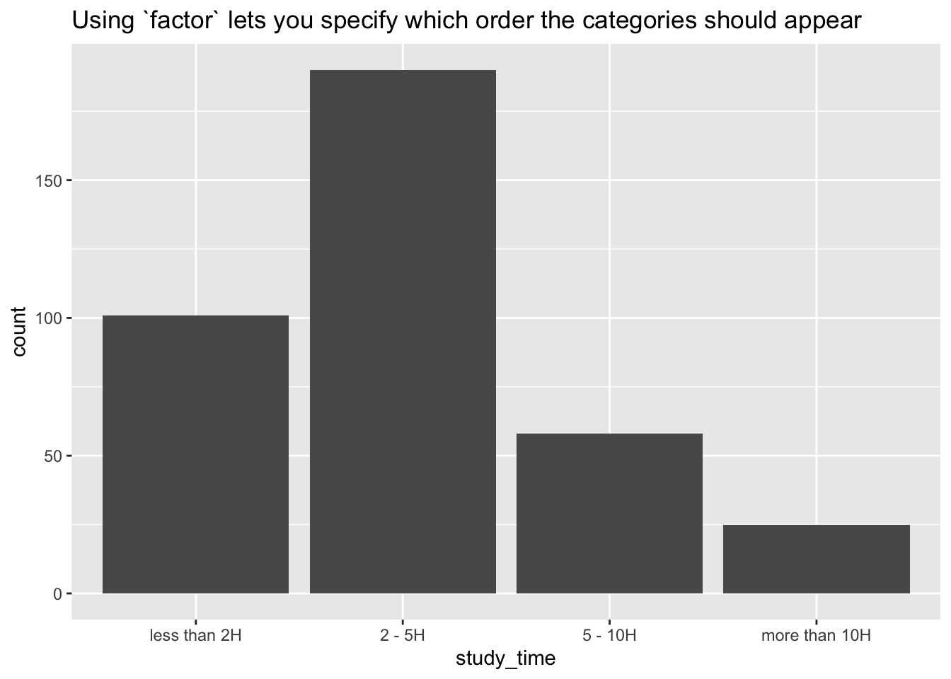
In order to avoid creating dummies by hand and to be able to choose the reference category yourself, I’d recommend using factor. The function factor takes a variable and coerces it to be a “factor” type, which is categorical. That variable can be ordered, and you can specify which level should go first, second, third, and so on. This is also useful for rearranging the categories of a variable in ggplot.
students %>%mutate(study_time =factor(study_time, levels =c("less than 2H", "2 - 5H", "5 - 10H", "more than 10H"))) %>%lm(final_grade ~ study_time, data = .) %>% broom::tidy()
students %>%mutate(study_time =factor(study_time, levels =c("less than 2H", "2 - 5H", "5 - 10H", "more than 10H"))) %>%ggplot(aes(x = study_time)) +geom_bar() +ggtitle("Using `factor` lets you specify which order the categories should appear")