3.8 Compensating Variation and Equivalent Variation

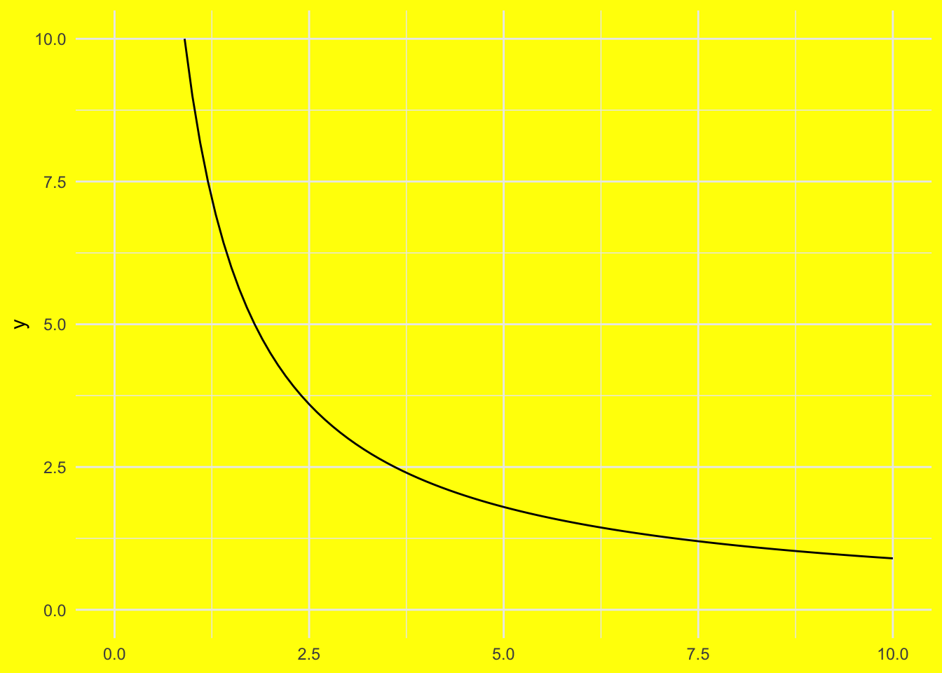
In this assignment, we’ll explore how Consumer’s Surplus (CS) serves as an approximation for two more precise measures of changes in consumer welfare: Compensating Variation (CV) and Equivalent Variation (EV). Using household expenditure data, we’ll analyze how changes in food prices impact consumer welfare.

The challenge with Consumer’s Surplus is that it assumes a dollar has the same value to a person, regardless of their purchasing power. For example, imagine a consumer spends 90% of their income on good 1. In this case, the Cobb-Douglas utility function would be a good fit: $u(x_1, x_2) = x_1^{.9}x_2^{.1}$.

Of course, the Cobb-Douglas trick tells us that the consumer will spend 90% of their income on good 1: $.9 m = p_1 x_1$. Solving for $x_1$ gets us the consumer’s demand function: $x_1 = \frac{.9 m}{p_1}$.

Now, suppose the price of good 1 increases from 1 to 2, and the consumer has an income of 10. The change in consumer’s surplus would be $6.24:

library(tidyverse)

ggplot() +
  stat_function(fun = function(x) .9 * 10 / x) +
  xlim(0, 10) +
  ylim(0, 10)

integrate(function(x) .9 * 10 / x, upper = 2, lower = 1)

6.238325 with absolute error < 6.9e-14

But how do we interpret this $6.24? Is it:

The amount we’d need to give someone after the price change to restore their original level of utility, or
The amount we could take away from someone before the price change that would make them just as happy as accepting the price change?

The difference is the reference point, and especially, the purchasing power the consumer has at each reference point. As it turns out, Consumer’s Surplus is neither of these. Instead, it’s a number that falls between the two measures but doesn’t have a precise interpretation on its own. The first measure is called Compensating Variation (CV), and the second is called Equivalent Variation (EV). These concepts help us better understand how price changes affect consumer welfare.

1) Household Expenditure Data

Run this code to get started: it attaches the tidyverse to your current session and then loads in a data set of consumer spending and income (both measured in british pounds per week).

library(tidyverse)

consumer <- read_csv("https://raw.githubusercontent.com/cobriant/320data/refs/heads/master/consumer.csv")

Edit the variable definition of consumer to include a new variable food_share that is equal to the share of total income the person spends on food.
Show that most people spend around 35% of their income on food, so using this Cobb-Douglas utility function is justified: $u(x_1, x_2) = x_1^{.35} x_2^{.65}$ where $x_1$ is the amount of food purchased and $x_2$ is the amount spent on all other things. Answer this question with summarize and then with a histogram.

Answer:

Does having kids change the proportion of income people spend on food?

Answer:

Does a person’s age change the proportion of income people spend on food?

Answer:

Find the median income for people in the data set (income is measured in british pounds per week).

Answer:

2) Cobb-Douglas Utility Function

In the previous section, we made an argument by looking closely at the data for why the utility function $u(x_1, x_2) = x_1^{0.35} x_2^{0.65}$ is justified here. Take that utility function and derive the demand function, using the median income for $m$.

Answer:

3) Compensating Variation

Using the demand function, fill out the table for $x_1$ and $x_2$, the amount of food purchased at different price levels, and the amount spent on all other things.

$m$	$p_1$	$p_2$	$x_1$	$x_2$
120	1	1	___	___
120	2	1	___	___

Answers:

$m$	$p_1$	$p_2$	$x_1$	$x_2$
120	1	1	___	___
120	2	1	___	___

Add one more column to the table: the utility the consumer gets from each bundle.

Answer:

Compensating variation answers this question: how much money would we have to compensate the consumer with after the price change to make them just as well off as before the price change? That is, under prices $p_1 = 2$ and $p_2 = 1$, find the income the consumer would need to get a utility of 62.8.

Answer:

4) Equivalent Variation

Equivalent variation answers the question the other way around: before the price change, how much money would we have to take away from the consumer for them to be just as well off as after the price change?

Answer:

Choosing between CV and EV

In general, CV and EV will yield different amounts because they have different reference points for utility: CV is grounded in the initial utility level, while EV is based on the final utility level. This divergence is not an error, but a feature of these measures.

Policymakers should use CV when they want to compensate consumers for a price change and restore them to their original level of utility. Alternatively, they should use EV when they want to evaluate willingness to accept a price change before it happens.