3.5 Choice

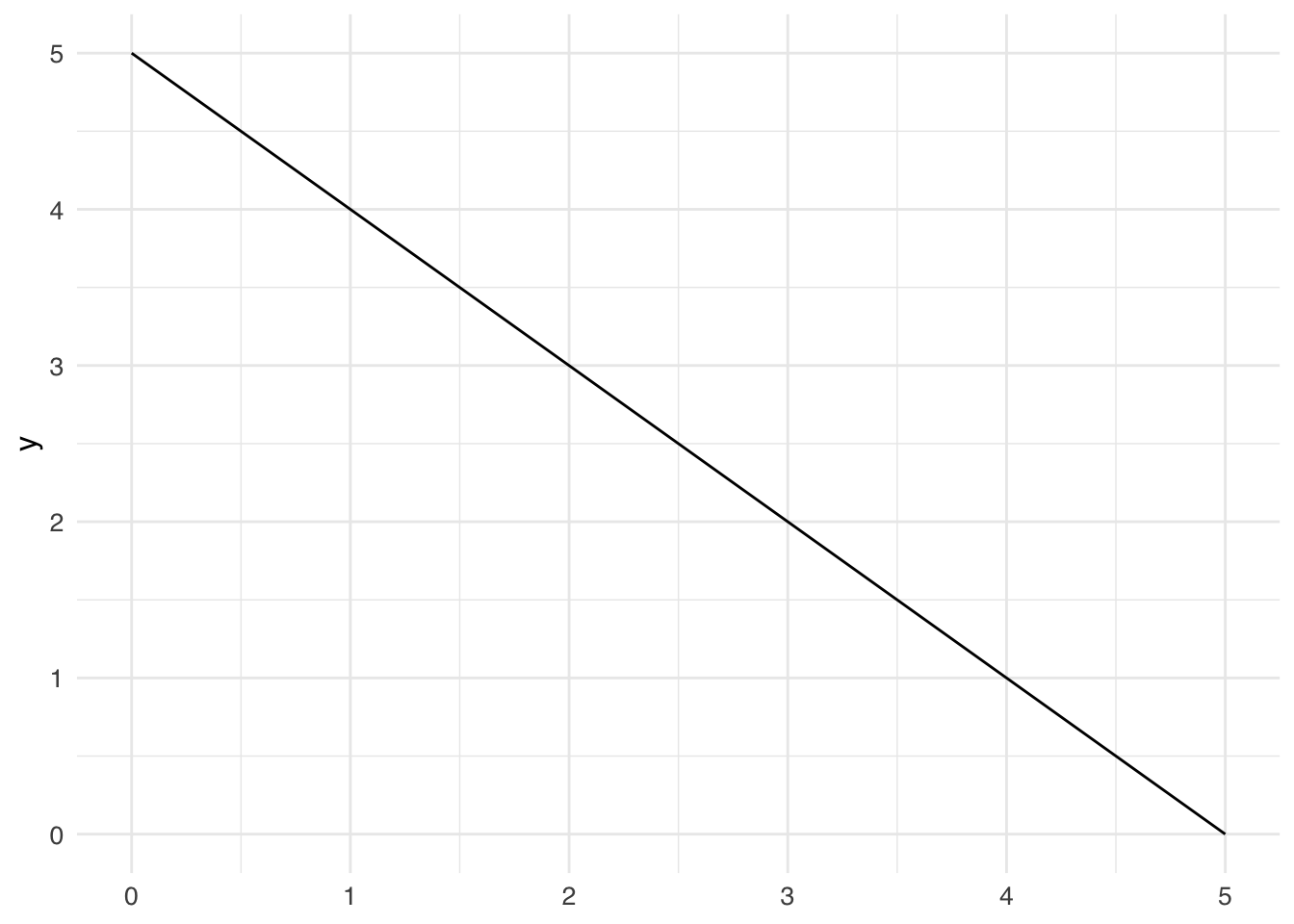
For more information on these topics, see Varian Chapter 5: Choice and Chapter 6: Demand.

In this chapter, you will combine the budget set and the theory of preferences to examine the choices of consumers. Earlier, I stated that the economic model of consumer choice is that people choose the best bundle they can afford. Now I can rephrase that more rigorously as, “consumers choose the most preferred bundle from their budget sets.”

Optimal Choice

I’ll plot the budget line $p_1 x_1 + p_2 x_2 = 5$ for the case where the price of both goods 1 and 2 are $1 and the consumer has an income of $5 to spend.

library(tidyverse)

ggplot() +
    stat_function(fun = function(x1) 5 - x1, color = "black") +
    xlim(0, 5)

Then I’ll add to that budget line: indifference curves of the utility function $u(x_1, x_2) = x_1 x_2$.

p <- ggplot() +
    stat_function(fun = function(x1) 5 - x1, color = "black") +
    stat_function(fun = function(x1) 2/x1, aes(color = "u = 2")) +
    stat_function(fun = function(x1) 4/x1, aes(color = "u = 4")) +
    stat_function(fun = function(x1) 6.25/x1, aes(color = "u = 6.25")) +
    stat_function(fun = function(x1) 8/x1, aes(color = "u = 8")) +
    xlim(0, 5) +
    ylim(0, 5) +
    geom_point(data = point_data, aes(x = x, y = y), color = "black", size = 3) +
    transition_reveal(along = -x)

animate(p)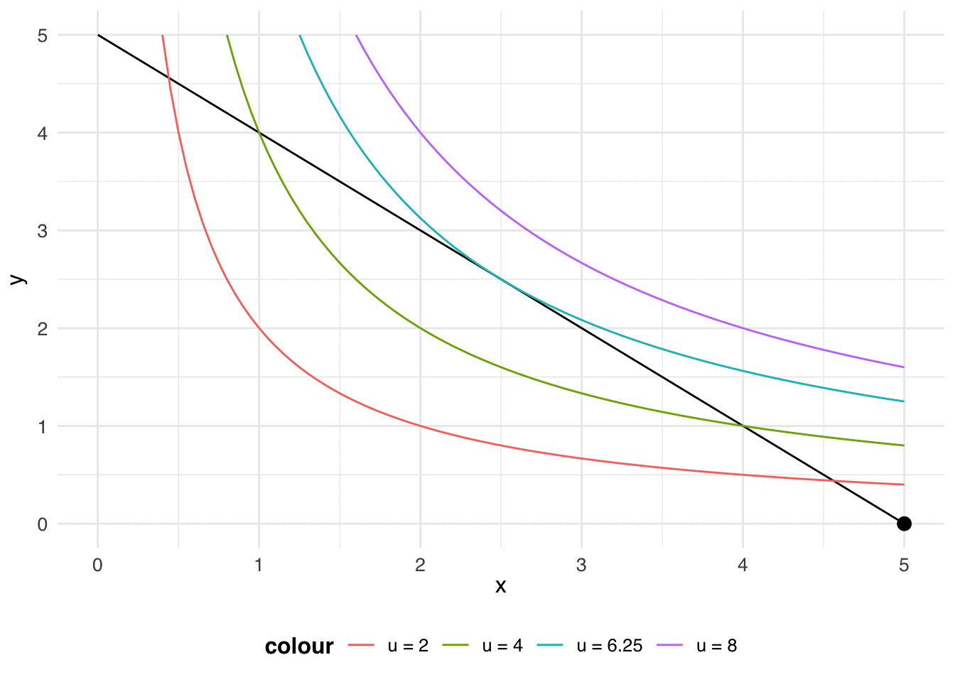

Let your eye follow the black dot along the budget line: along that line, the consumer exhausts their income on goods 1 and 2. The budget line crosses the red indifference curve ($u = 2$), so you know that the consumer can get more than a utility of 2. The budget line also crosses the green indifference curve ($u = 4$), so you know that the consumer can get more than a utility of 4. Something interesting happens at the blue indifference curve ($u = 6.25$): the budget line doesn’t cross the blue indifference curve, the budget line is tangent to the blue indifference curve. The point of tangency represents the bundle that will earn the consumer the highest utility ($u = 6.25$), while still being affordable.

The point of tangency represents the most preferred bundle from the consumer’s budget set: this is the consumer’s choice.

When two lines are tangent to each other, they have the same slope. That is, at the consumer’s choice, the slope of the budget line ($\frac{-p_1}{p_2}$) is equal to the slope of the indifference curve (-MRS = $-\frac{\frac{\partial u}{\partial x_1}}{\frac{\partial u}{\partial x_2}}$). We’ll use this fact to solve for the consumer’s choice given a budget constraint and a utility function.

Exercise 1

Consider the utility function: $u(x_1, x_2) = x_1^{0.5} x_2^{0.5}$. This is a monotonic transformation of the $u(x_1, x_2) = x_1 x_2$ utility function that we’ve explored a couple of times, so indifference curves are the well behaved ones we’re used to seeing. Take another monotonic transformation (natural log) to see that $u(x_1, x_2) = 0.5 \ln x_1 + 0.5 \ln x_2$: I’ll do this to make $u$ easier to work with. If the optimal bundle is an interior point, then we have 2 equations:

Equation 1: $-MRS = \frac{-p_1}{p_2}$, where $MRS = \frac{\ \partial u(x_1, x_2)/\partial x_1}{\partial u(x_1, x_2) / \partial x_2}$.
Equation 2: The consumer’s choice is on the budget line: $p_1 x_1 + p_2 x_2 = m$. Let $p_1 = 1$ and $p_2 = 1$, and income $m = 5$.

We have 2 unknowns: $x_1$ and $x_2$. Use the 2 equations to solve for the 2 unknowns: you should get $x_1 = 2.5$ and $x_2 = 2.5$. This is the same problem as the problem depicted in the animation above.

Answer: \[\begin{align} \end{align}\]

Cobb-Douglas Trick

Here’s a shortcut for solving problems like exercise 1: if you can put the utility function in the form of a Cobb-Douglas utility function, you can skip a lot of that algebra.

A Cobb-Douglas utility function is a utility function of the form $u(x_1, x_2) = x_1^a x_2^b$, where $a$ and $b$ are non-negative and $a + b = 1$. This type of utility function has a useful property where the exponents $a$ and $b$ tell you the share of the consumer’s income that will be spent on goods 1 and 2 at the consumer’s optimal bundle. For example, in exercise 1, the exponents were (0.5, 0.5). You can solve exercise 1 using the Cobb-Douglas trick like this:

The Cobb-Douglas utility function is $u(x_1, x_2) = x_1^{0.5} x_2^{0.5}$. This tells us that the consumer will choose to spend 50% of their income on good 1: $p_1 x_1 = .5 m$, and 50% of their income on good 2: $p_2 x_1 = .5 m$.
Plug in the price of goods 1 and 2 along with the consumer’s income: ($p_1 = 1$, $p_2 = 1$, $m = 5$).
You’ll get that $1 x_1 = .5 (5)$ and $1 x_2 = .5 (5)$, and simplify: $x_1 = 2.5$ and $x_2 = 2.5$.

Exercise 2

Use the Cobb-Douglas trick to find the consumer’s choice if their utility function is $u(x_1, x_2) = x_1^{.25}x_2^{.75}$, $p_1 = 1$, $p_2 = 2$, and $m = 12$.

Answer: \[\begin{align} \end{align}\]

Exercises 3 and 4 will give you more practice solving for the consumer’s choice.

Exercise 3

Use the tangency condition and budget constraint to solve for the consumer’s choice given $u(x_1, x_2) = x_1^{1/3}x_2^{2/3}$, $p_1 = 1$, $p_2 = 2$, and $m = 3$. Then check your work by using the Cobb-Douglas trick.

Answer using the tangency condition and budget constraint: \[\begin{align} \end{align}\]

Answer using Cobb-Douglas trick: \[\begin{align} \end{align}\]

Exercise 4

Use the tangency condition and budget constraint to solve for the consumer’s choice given $u(x_1, x_2) = x_1^{4/5}x_2^{1/5}$, $p_1 = 2$, $p_2 = 2$, and $m = 10$. Then check your work by using the Cobb-Douglas trick.

Answer using the tangency condition and budget constraint: \[\begin{align} \end{align}\]

Answer using Cobb-Douglas trick: \[\begin{align} \end{align}\]

Demand Curves

A demand curve tells you what a consumer’s demand for good 1 is at any possible $p_1$. If we can derive the consumer’s choice, we can also derive the consumer’s demand curve.

Exercise 5

Use the Cobb-Douglas trick to solve for the consumer’s choice given $u(x_1, x_2) = x_1^{.5} x_2^{.5}$, $p_2 = 1$, and $m = 10$. Leave $p_1$ as a variable: your final answer for $x_1$ should be a function of $p_1$. What you’ve derived is the consumer’s demand curve for good 1.

Answer using Cobb-Douglas trick: \[\begin{align} \end{align}\]

Exercise 6

Use ggplot to plot the demand curve you derived in exercise 5. Put $x_1$ on the x-axis and $p_1$ on the y-axis. Does the law of demand hold here? That is, when $p_1$ falls, does the consumer choose to buy more of good 1?

Answer: