library(tidyverse)

weather <- read_csv("https://raw.githubusercontent.com/cobriant/teaching-datasets/refs/heads/main/world_weather.csv") %>%
  mutate(
    country = case_when(
      city == "Amsterdam"      ~ "NETHERLANDS",
      city == "Athens"         ~ "___",
      city == "Bangkok"        ~ "THAILAND",
      city == "Brussels"       ~ "BELGIUM",
      city == "Buenos Aires"   ~ "ARGENTINA",
      city == "Copenhagen"     ~ "DENMARK",
      city == "Dublin"         ~ "___",
      city == "Helsinki"       ~ "FINLAND",
      city == "Istanbul"       ~ "TURKEY",
      city == "Johannesburg"   ~ "SOUTH AFRICA",
      city == "Kuala Lumpur"   ~ "MALAYSIA",
      city == "London"         ~ "___",
      city == "Madrid"         ~ "SPAIN",
      city == "Manila"         ~ "PHILIPPINES",
      city == "Milan"          ~ "___",
      city == "New York"       ~ "UNITED STATES",
      city == "Oslo"           ~ "NORWAY",
      city == "Paris"          ~ "___",
      city == "Rio de Janeiro" ~ "BRAZIL",
      city == "Santiago"       ~ "CHILE",
      city == "Singapore"      ~ "SINGAPORE",
      city == "Stockholm"      ~ "SWEDEN",
      city == "Sydney"         ~ "___",
      city == "Vienna"         ~ "AUSTRIA",
      city == "Zurich"         ~ "SWITZERLAND",
      TRUE ~ NA_character_
    )
  )

stocks <- read_csv("world-stocks.csv")11 Hirshleifer and Shumway 2003 Part 2: Replication
Part 1: Data and Join
Read in the two data sets (one is from my github site; the other is from your own computer from classwork 10).
We need to join these two. Problem is: weather has only cities (“Amsterdam”); stocks has only countries (“NETHERLANDS”). We’ll have to use case_when to add a country variable to weather. Then we can join by country and date.
Question 1: Finish the case_when to add a variable country to the weather tibble.
Question 2: Join weather with stocks to create a new data set, joined_data.
joined_data <- ___Part 2: Visualize the Main Results
Question 3: Visualize the relationship between clouds and ret. Add a line of best fit. Then visualize that relationship separately for each country, using facet_wrap.
Part 3: Estimate the OLS Results

# Question 4:
# Regression A (red): pooled OLS regression. Use lm to estimate
# `ret ~ clouds`. Interpret: When clouds increase by 1 unit,
# returns are ____ (lower/higher), and that effect (is/is not)
# statistically significant at the 5% level.

joined_data %>%
  lm(___, data = .) %>%
  broom::tidy()

# Question 5:
# Regression B (yellow): separate OLS regressions for each country.
# Use `map` to map over every country in the data set and estimate
# `ret ~ clouds` with lm for every country.
countries <- joined_data %>%
  filter(!is.na(clouds), !is.na(ret)) %>%
  distinct(country) %>%
  pull(country)

ols_results <- map(
  ___,
  function(x) {
    ___ %>%
      ___(___) %>%
      lm(___, data = .) %>%
      broom::tidy() %>%
      filter(term == "clouds") %>%
      mutate(country = x, signif = abs(___) > 1.96) %>%
      select(country, estimate, statistic, signif)
  }
) %>%
  bind_rows()

view(ols_results)
ols_results %>% count(estimate < 0)

# Question 6: Interpret the results from question 5.
# There were 23 countries, and we found a negative coefficient
# on clouds ___ times and a positive coefficient on clouds ___
# times.
# If cloudiness had no real effect on stocks, what's the
# probability we'd see this many negative coefficients just
# by chance?
# To answer this question, run an experiment:
# Use `sample()` to simulate flipping a coin (TRUE or FALSE) 23 times.
# Did you get 9 or fewer TRUE's?
# Then use `map()` to repeat the experiment 100,000 times.
# How many times out of 100,000 did you get 9 or fewer TRUE's?

sum(sample(c(___, ___), size = ___, replace = ___)) <= 9

map(
  1:100000,
  function(x) sum(sample(c(___, ___), size = ___, replace = ___)) <= 9
) %>%
  as_vector() %>%
  mean()

# Another way to solve the problem, using the binomial distribution:
pbinom(q = 9, size = 23, prob = .5)
Part 4: Estimate the Logit Results
In OLS, we’re used to modeling continuous dependent variables like ret, which can take on any value:
ret ~ clouds
But sometimes the outcome is not continuous, it’s discrete (categorical), like the binary outcome TRUE/FALSE (or 1/0). In Hirshleifer and Shumway (2003), along with using OLS, they also ask whether cloudiness predicts the probability that returns are positive:
ret > 0 ~ clouds
That calls for a model designed for a discrete dependent variable, like a logit.
Discrete outcomes and the goal
A binary outcome can be written as:
\[y_t \in \{0, 1\}\] For example, \(y_t = 1\) if day \(t\) has a positive return, and 0 otherwise.
A logistic regression gives a predicted probability:
\[p_t = P(y_t = 1 | x_t)\]
Where \(x_t\) is the predictor (like clouds).
The problem with using OLS for discrete dependent variables
A tempting first step is to use OLS to fit a linear probability model:
\[\hat{p}(x_t) = \beta_0 + \beta_1 x_t\]
The linear probability model is intuitive, but it has two shortcomings: (1) it can easily predict nonsensical probabilities (p < 0 and p > 1), and (2) when x increases by 1, the predicted probability must increase linearly: it’s very restrictive.
Let’s work an example with the Love Island data set from Classwork 4:
library(tidyverse)

love <- read_csv("https://raw.githubusercontent.com/cobriant/320data/master/love.csv") %>%
  mutate(win = if_else(outcome %in% c("winner", "runner up", "third place"), 1, 0))

# Notice that it predicts probabilities outside the [0, 1] range.
love %>%
  ggplot(aes(x = age, y = win)) +
  geom_jitter(width = .1, height = .1) +
  geom_smooth(method = lm, se = F, fullrange = T) +
  labs(title = "Linear Probability Model") +
  xlim(0, 50)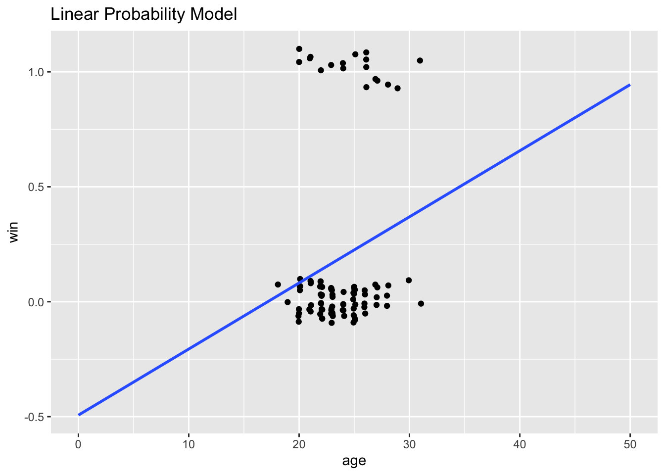
# Estimate the linear probability model:
love %>%
  lm(win ~ age, data = .) %>%
  broom::tidy()
# A tibble: 2 × 5
term estimate std.error statistic p.value
<chr> <dbl> <dbl> <dbl> <dbl>
1 (Intercept) -0.493 0.351 -1.41 0.163
2 age 0.0288 0.0147 1.95 0.0539The predicted probability that someone who is age 0 wins the show is -0.493: a nonsensical value for a probability.
Instead, here’s what a logit looks like. Notice that it predicts probabilities bounded by 0 and 1, and lets marginal effects be nonlinear:
love %>%
  ggplot(aes(x = age, y = win)) +
  geom_jitter(width = .1, height = .1) +
  geom_smooth(method = "glm", method.args = list(family = "binomial"), se = F, fullrange = T) +
  labs(title = "Logit") +
  xlim(0, 50)
`geom_smooth()` using formula = 'y ~ x'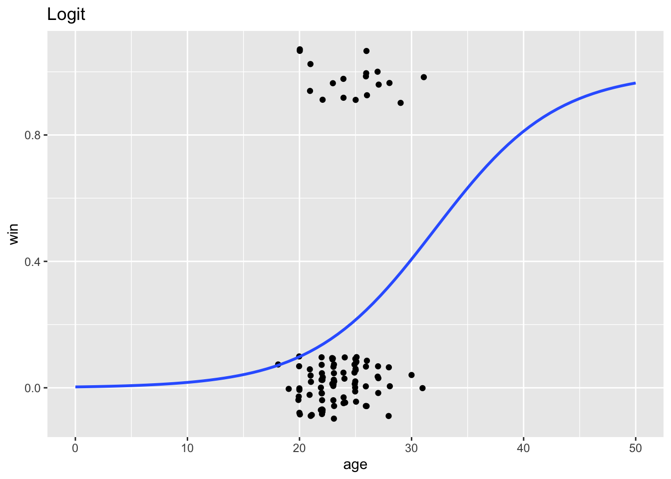
What is a logit?
A logit starts with the odds of an outcome happening: \(\frac{p(x)}{1 - p(x)}\), and then takes the natural log of those odds.
It assumes the model is linear in log-odds: \(\log\left(\frac{p(x)}{1 - p(x)}\right) = \beta_0 + \beta_1 x\), which makes it curved in probability.
Interpreting Logit Results
Take the love island logit:
love %>%
  glm(win ~ age, data = ., family = "binomial") %>%
  broom::tidy()
# A tibble: 2 × 5
term estimate std.error statistic p.value
<chr> <dbl> <dbl> <dbl> <dbl>
1 (Intercept) -5.90 2.40 -2.46 0.0140
2 age 0.184 0.0975 1.89 0.0593We estimate \(\beta_0 = -5.9\) and \(\beta_1 = 0.184\). Taking the equation \(\log\left(\frac{p(x)}{1 - p(x)}\right) = \beta_0 + \beta_1 x\), we can rearrange and solve for \(p(x)\): \[p(x) = \frac{1}{1 + e^{-(\beta_0 + \beta_1 x)}}\]
Next, let \(\beta_0 = -5.9\) and \(\beta_1 = 0.184\):
p <- function(age) 1/(1 + exp(-(-5.9 + .184 * age)))

# Someone who is 0 years old has a chance of winning of:
p(0)
[1] 0.002731961# Someone who is 20 years old has a chance of winning of:
p(20)[1] 0.0979688# Someone who is 25 years old has a chance of winning of:
p(25)[1] 0.214165# Someone who is 30 years old has a chance of winning of:
p(30)[1] 0.4061269Back to the replication
Question 7: Estimate the logit positive_return ~ clouds for the entire data set, and then for each country separately. Just like with OLS, the estimate we’re most interested in is still the coefficient on clouds and its statistical significance.
# Regression C (green): pooled logit
joined_data %>%
  mutate(positive_return = ret > 0) %>%
  glm(___, data = ., family = "binomial") %>%
  broom::tidy()

# Regression D (blue): separate logit estimates for each country
logit_results <- map(
  ___,
  function(x) {
    ___ %>%
      ___(___) %>%
      ___(___) %>%
      glm(___, data = ., family = "binomial") %>%
      ___ %>%
      ___(term == ___) %>%
      ___(country = x, signif = abs(___) > 1.96) %>%
      select(country, estimate, statistic, signif)
  }
) %>%
  bind_rows()

view(logit_results)
logit_results %>% count(estimate < 0)
Question 8: Interpret. Did the results from this paper hold up to replicating it for data from 2015 to 2025 versus the paper’s date range (1982 to 1997)?
Download this assignment
Here’s a link to download this assignment.