8 DeBondt and Thaler (1985) Replication

Part 1: Data

Hopefully your WRDS account has been approved. Sign in and navigate to Get Data > CRSP > Annual Update > Stock / Security Files > Monthly Stock File.

Fill out the query form like this:

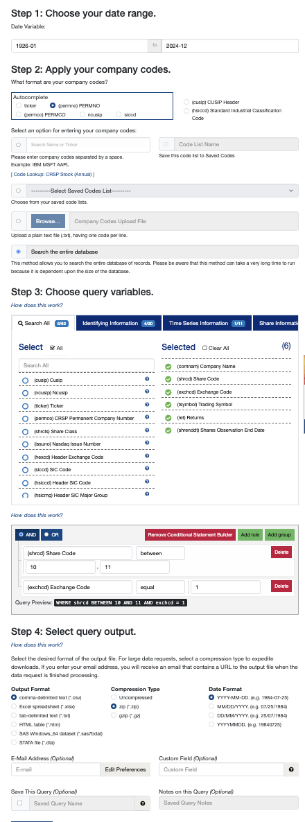
It should take about 30 seconds to complete. Check to make sure you got 1,423,668 rows. Then you can download your zip file and extract it.

library(tidyverse)

stocks <- read_csv("___") %>%
  select(permno = PERMNO, date, ret = RET, company = COMNAM) %>%
  mutate(ret = as.double(ret))

Variables

permno: a permanent number that uniquely identifies a security throughout time, even when branding changes.

date: “YYYY-MM-DD”: the last trading day of the month.

ret: the stock’s return on that date.

company: company name. With mergers, bankruptcies, and relistings, company names and trading symbols might change, but PERMNO will not. If you owned shares of Google in 2015, they automatically became shares of Alphabet overnight.

Question 1: Exploring the data with dplyr

Answer each of these questions with dplyr queries:

• 1. How many unique stocks (permno) are in this data set?
• 2. Which 10 stocks had the highest returns, and when did they occur?
• 3. Which 10 stocks had the lowest returns, and when did they occur?

Question 2: Exploring the data with ggplot2

Answer each of these questions with a ggplot:

• 1. Visualize a time series of the gamestop returns.
• 2. Visualize the COVID crash, centered on April 2020.
• 3. Visualize the 2008 crisis, centered on November 2008.

Part 2: The Replication

Question 3: Instead of using raw returns, DeBondt and Thaler compute the residual (excess) return for a stock at a given month as u = return - equal weighted market return. An equal weighted market return is just the average return for that month across the entire data set. Edit the original variable definition of stocks to create a new variable ret_resid. Ungroup at the end so that the grouping attributes you formed don’t carry over into the rest of the project. View the data set afterward to make sure ret_resid looks how you would expect.

Then run the code in this chunk before moving forward:

# This enforces D&T's rule "once a stock has a missing
# return, treat it as dead (NA) forever". It will remove
# small, less established firms from the data set.
# `cumany` is a cumulative function: it will apply NA to 
# all cases after the first NA appears.

stocks <- stocks %>%
  group_by(permno) %>%
  mutate(ret_resid = if_else(cumany(is.na(ret_resid)), NA_real_, ret_resid)) %>%
  ungroup()

Question 4: Pre-Period: Form Winner and Loser Portfolios in January 1933

We’ll form “winner” and “loser” portfolios by looking at data from the pre-period: the three years between January 31, 1930 and December 31, 1932. The 35 stocks with the highest return sum in that three-year period become our “winner” portfolio in January 1933; the 35 stocks with the lowest return sum become our “loser” portfolio.

Start by filtering for only stocks in this 3-year pre-period. Add together the returns for each stock in the pre-period.

Winners are the 35 with the highest pre-period return sum; losers are the 35 with the lowest.

t0 <- ymd("1932-12-31")

stocks %>%
  filter(
    date > t0 %m-% months(36),
    date <= t0 %m-% months(1),
    !is.na(ret_resid)
    ) %>%
  # n_months: if the stock has any NAs in the pre-period, it's dropped.
  group_by(permno) %>%
  summarize(pre_pd_sum = sum(___), n_months = n()) %>%
  filter(n_months == 35) %>%
  arrange(___) %>%
  mutate(portfolio = c(rep("W", 35), rep("middle", n() - 70), rep("L", 35))) %>%
  filter(portfolio != "middle")

Question 5: Post-Period: Compute 3-Year Cumulative Average Residual Returns for the Portfolio

Add to your query from question 4. Take the winners and losers and use left_join to fill in return information for the post-period: the 3 years after the portfolio is formed.

Calculate the portfolio return for winners and losers each month after the portfolio formation. portfolio_cumsum will be a cumulative sum of the winner portfolio returns and loser portfolio returns.

t0 <- ymd("1932-12-31")

stocks %>%
  filter(
    date > t0 %m-% months(36),
    date <= t0 %m-% months(1),
    !is.na(ret_resid)
    ) %>%
  group_by(permno) %>%
  # n_months: if the stock has any NAs in the pre-period, it's dropped.
  summarize(pre_pd_sum = sum(___), n_months = n()) %>%
  filter(n_months == 35) %>%
  # The winner portfolio is formed with the stocks that did the best
  # in the pre-period; the loser portfolio is formed with the stocks
  # that did the worst.
  arrange(___) %>% 
  mutate(portfolio = c(rep("W", 35), rep("middle", n() - 70), rep("L", 35))) %>%
  filter(portfolio != "middle") %>%
  # Now we look at how these winners and losers did throughout the
  # post-period: the 3 years after portfolio formation.
  left_join(
      filter(stocks, ___ >= t0 %m+% months(1),
             ___ <= t0 %m+% months(36))) %>%
  select(permno, portfolio, date, ret_resid) %>% 
  group_by(___, ___) %>%
  summarize(portfolio_return = mean(___, na.rm = T)) %>% 
  # For comparing between different formation dates, 
  # translate dates to months after formation
  mutate(month = 12 * (year(date) - year(t)) + (month(date) - month(t))) %>%
  group_by(portfolio) %>%
  mutate(portfolio_cumsum = cumsum(___))

Question 6: Form Portfolios Every 3 Years

The hard parts are over! Now, we don’t only want to form these portfolios in January 1933, we want to form portfolios every three years until 1977.

Copy-paste your code from question 5 into map(), where the .x we’ll iterate over are the portfolio formation dates, and the .f is a function that takes a portfolio formation date t and returns a tibble with the portfolio (W or L), the month after portfolio formation (1 to 36), and the portfolio_cumsum.

t0 <- ymd("1932-12-31")
map(
  .x = seq.Date(from = t0, to = ymd("1977-12-31"), by = "3 years"),
  .f = function(t) {
    
  }
) %>%
  bind_rows()

Question 7: Visualize Your Results

After the map() call in question 6, average portfolio_cumsum for each portfolio (W or L) and each month (1 to 36), and visualize the results with average portfolio cumsum on the y-axis and month after portfolio formation on the x-axis, with color representing the portfolio (W or L).

Did we get close to DeBondt and Thaler’s Figure 1?

Question 8: Form Portfolios at a Different Time of Year

Are the results sensitive to the January portfolio formation decision? Try it all again with different starting months.

t0 <- ymd("1932-12-31") %m+% months(5)
map(
  ___
) %>%
  bind_rows() %>%
  ___

Question 9: New Data

Instead of forming portfolios in 1933, let’s shift everything forward 47 years, to consider the most recent data we can. Do we still see the same reversal pattern? What about when we only focus on the past 30 years?

t0 <- ymd("1932-12-31") %m+% years(47)
map(
  ___
) %>%
  bind_rows() %>%
  ___

Download This Assignment

Here’s a link to download this assignment.

Jegadeesh and Titman (1993) and Da, Engelberg, and Gao (2011) Discussion Questions

Over the weekend, read these two papers and prepare for Monday’s discussion by responding to these prompts, uploading your responses to Canvas before class on Monday.