library(tidyverse)6 Omitted Variable Bias
Groupmates present: ___________________
We learned that, in the regression \(y_i = \beta_0 + \beta_1 x_i + u_i\), the estimator for \(\beta_1\) is \(\frac{\text{Cov}(x, y)}{\text{Var}(x)}\): it’s a measure of the correlation between \(x\) and \(y\). So there are issues with and assumptions we need to make when we interpret \(\beta_1\) as the effect of a change in \(x\) on \(y\). That is, is \(\beta_1\) correlation or is it causation? In this classwork, we’ll explore those issues and assumptions.
The Earnings-Education Question
The field of Education Economics is concerned with, more than anything else, this regression:
\[\text{Earnings}_i = \beta_0 + \beta_1 \text{Education}_i + u_i\]
Take any dataset, around the world, throughout history, add as many other explanatory variables as you like (field, industry, gender, experience, parent’s education, etc) and you’ll find that the years someone spends in school seems to have an incredibly large and positive effect on their earnings down the road. And that makes sense: education should give you the skills and the new ways of thinking that ensure you’ll be successful in the real world. If it didn’t, what would be the point?
The thing is, the size of that \(\hat{\beta}_1\) is so large and positive that you have to wonder: if education is such a good investment, why do so many people drop out of high school? Why do so many people not go to college (when the cost of student loans is miniscule compared to the boost you seem to get to lifetime earnings)? Why do so many people drop out of college? As economists, we don’t usually like to chalk things up to irrational behavior. There has to be something else going on!
The answer is that there is omitted variable bias in that regression. There are variables that are really, really important in determining someone’s earnings, those variables are really hard to measure, and those variables are also highly correlated with how much education someone has received. They are: ability, conscientiousness, and conformity.
High ability people get more education because school is easy for them, and then they go on to have successful careers, but not necessarily because of their educations. Very conscientious people turn in better assignments both in school and at work. People who are conformists are more likely to stay in school and get along better in the workplace.
There’s no good way to measure ability, conscientiousness, and conformity, so when we have to leave them out of the earnings ~ education regression, because they’re correlated so strongly with both earnings and education, they confound the earnings-education relationship we’re trying to understand. What if it’s not because someone has so much education that they’re successful; what if it’s because they have a high ability, they’re very conscientious, or they’re a conformist? Given only observational data on people’s salaries and educations, we can never know which one it is.
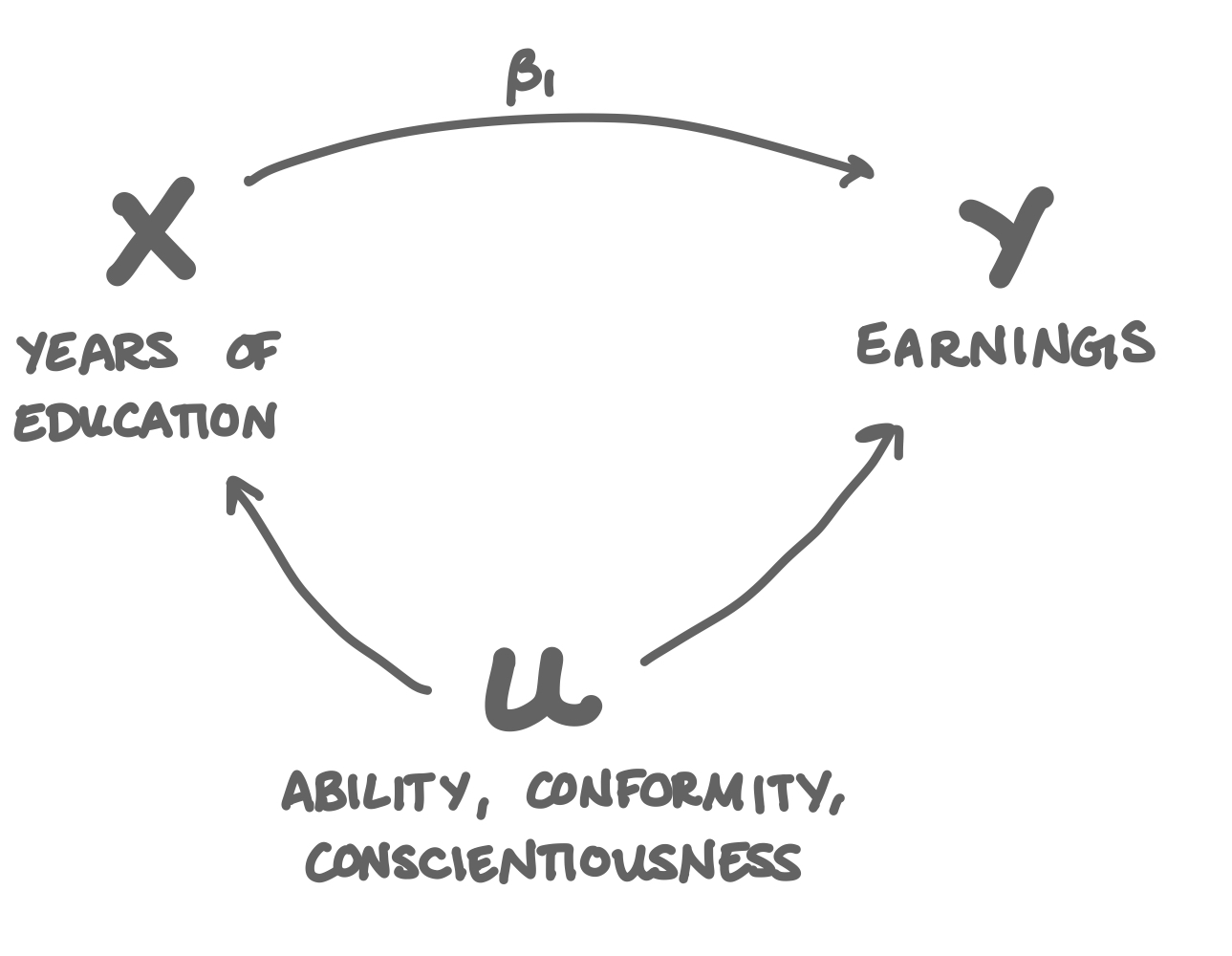
When we have to omit ability, conscientiousness, or conformity from that earnings-education model, we can’t tell whether someone’s high earnings is because of their education, or because of their high ability, conscientiousness, or conformity. As a result, education always appears to be a much better investment than it probably actually is.
Question 1
A variable \(z\) that is aborbed into \(u\) confounds the relationship between \(x\) and \(y\) if:
- \(z\) affects \(x\)
- \(z\) affects \(y\)
- \(z\) affects \(x\) or \(z\) affects \(y\)
- \(z\) affects \(x\) and \(z\) affects \(y\)
Question 2
Suppose you’re trying to understand how the number of opposite sex friends someone has effects their high school GPA (perhaps to make a case for or against same-sex schools). The thing is, you have to omit how strict the students’ parents are from the regression because there’s no good measure of that variable. Will omitting “strictness of parents” add bias, and why?
Simulations
Simulations can be a really powerful tool in empirical work to learn more about the properties of estimators and when to expect biased results. In this section, you’ll do a number of simulations considering the relationships between these three variables: earnings, education, and ability. You will simulate the data generating process and then you’ll consider, out of all possible regressions you could run, which would give you unbiased estimates of the causal effects, and which would not.
Hints:
- When your dependent variable (y) has an effect on any of your explanatory variables, you’re in trouble. It should be the other way around.
- Look for omitted variable bias in at least one of these regressions. You’ll find OVB when X <- U -> Y.
- When X -> Y and X -> U -> Y, you’ll get unbiased estimates with Y ~ X. The thing that’s going on here is that U is a “mediator”: X has a direct effect on Y (X -> Y), and X also has an indirect effect on Y (X -> U -> Y). The entire effect of X on Y is the direct effect plus the indirect effect, and OLS estimates it.
- 3/9 of these models yield unbiased coefficient estimates.
- Your simulation should start with this: generate a synthetic data set with 3 variables: ability, education, and earnings. Ability should be random uniform:
runif. Education should be a linear function of ability with some random noise, generated withrnorm. Then earnings should be a linear function of both education and ability, also with some random noise (rnorm) added on. - After you generate a synthetic data set, use
lmto estimate a model and usebroom::tidy(), select, and slice to find the estimate for \(\beta_1\). - Run the simulation perhaps 100 times, saving the estimate for \(\beta_1\) each time. Use
map(.x, .f)for this task. Draw ageom_histogramplot with a vertical line (geom_vline) for the true effect of \(x_1\) on \(y\). Then interpret your simulation results by discussing whether or not OLS seems to be unbiased.
Question 3
Run simulations for each of these models, producing a histogram plot of simulation results for each. Then interpret your findings: is \(\hat{\beta}_1\) a biased or unbiased estimate of the true causal effect of \(x_1\) on \(y\)?
1. \(Earnings_i = \beta_0 + \beta_1 Education_i + \beta_2 Ability_i + u_i\)
2. \(Earnings_i = \beta_0 + \beta_1 Education_i + u_i\)
3. \(Earnings_i = \beta_0 + \beta_1 Ability_i + u_i\)
4. \(Education_i = \beta_0 + \beta_1 Ability_i + \beta_2 Earnings_i + u_i\)
5. \(Education_i = \beta_0 + \beta_1 Ability_i + u_i\)
6. \(Education_i = \beta_0 + \beta_1 Earnings_i + u_i\)
7. \(Ability_i = \beta_0 + \beta_1 Education_i + \beta_2 Earnings_i + u_i\)
8. \(Ability_i = \beta_0 + \beta_1 Education_i + u_i\)
9. \(Ability_i = \beta_0 + \beta_1 Earnings_i + u_i\)
Extra Credit
Programmers like to say DRY: “don’t repeat yourself”.
You may notice that your simulations contain a lot of repeated code. Why is this problematic? Recall that one of our main goals when it comes to programming is to write code that’s clear and readable. When you have a lot of code that’s copy-pasted over and over, it’s less clear and harder to read. Code that’s hard to read also has the problem that if there’s a mistake, it’s harder to catch. So your challenge is to write a function simulation that takes a model as a character string and a true_beta1 value to draw the vertical line. You should be able to call your function more or less like this:
simulation(model = "earnings ~ education + ability", true_beta1 = 1)
And your function should return a histogram of the simulation results. After writing simulation, hopefully you can go back through and remove all of your repeated code.
Download this assignment
Here’s a link to download this assignment.
There is no autograder for this one: compile your document to html and submit the html file to Canvas (one copy per group).