library(tidyverse)

google <- read_csv("https://raw.githubusercontent.com/cobriant/FEARS/refs/heads/main/FEARS.csv")

sp500 <- read_csv("___")9 Da, Engelberg, and Gao (2015) Replication
In this assignment, you will replicate the key empirical result from Da, Engelberg, and Gao (2015): The Sum of All FEARS: Investor Sentiment and Asset Prices.
The core idea: a spike in fear-related google searches is predictive of markets falling immediately, and then reversing in subsequent days.
Data
For this replication, we’ll start with 2 data sets:
- Google search volume for 30 keywords like “bankrupt”, “crisis”, “benefits”, and “unemployment” (daily hits for each keyword, July 1 2004 to Dec 31 2011)
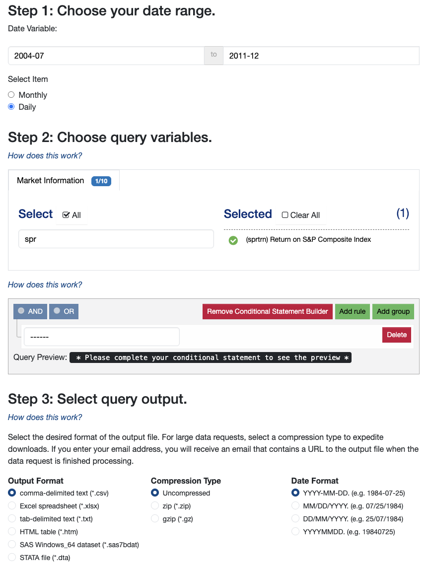
- CRSP data for the S&P500 composite index return series (not individual stocks, daily, July 1 2004 to Dec 31 2011)
I’ve prepared the first data set for you. The second you’ll get from WRDS:
CRSP > Annual Update > Stock/Security Files > Stock Market Indexes
Key skills
lag and lead
In time series data, we often compare things like data from today to:
- data from yesterday
- data from tomorrow
- data from 2 days ahead
- etc.
That’s what lag() and lead() do.
# Example:
tibble(
  x = 1:10
) %>%
  mutate(
    lag = lag(x),
    lag2 = lag(x, 2),
    lead = lead(x),
    lead2 = lead(x, 2)
)lag(x)shifts the vector down by 1.lag(x, 2)shifts it down by 2.lead(x)shifts the vector up by 1.lead(x, 2)shifts it up by 2.
Question 1: Suppose ret is the daily return of the S&P 500. Create a new variable called ret_change that measures the change in returns from yesterday to today: \(\mathrm{ret\_change} = ret_t - ret_{t-1}\). Then create a variable ret_next_change that measures how much returns change from today to tomorrow: \(\mathrm{ret\_next\_change} = ret_{t+1} - ret_{t}\).
tibble(
  day = 1:10,
  ret = rnorm(n = 10, mean = 0, sd = .01)
) %>%
  mutate(
    ret_change = ___,
    ret_next_change = ___
    )
Joins: left_join, inner_join, and full_join
left_join joins two tables, keeping all rows that are in the left hand tibble and filling them out with information gained from the right hand tibble.
# Example data
sales <- tibble(day = 1:10, sales = runif(0, 100, n = 10))
weather <- tibble(
  day = 5:14,
  weather = sample(c("sunny", "rainy"), size = 10, replace = T)
)

# left_join will keep only rows that show up in the left hand tibble:
# sales. So this query will keep days 1-10:
sales %>%
left_join(weather, join_by(day))inner_join, on the other hand, keeps only rows that are in both tables:
# returns data for days 5:10
sales %>%
  inner_join(weather, join_by(day))
full_join keeps any row that is in either table:
# returns data for days 1:14
sales %>%
  full_join(weather, join_by(day))
Question 2: Suppose your left hand table has data from all days, including weekends. And your right hand table has data only from weekdays. Explain whether weekends will be in the result if you use a left_join, an inner_join, and a full_join.
dplyr and ggplot2
Question 3: Draw a time series of the S&P500 returns. What stands out and how might this date range choice affect the results in this paper?
Question 4: Draw a time series for the google search volume for the keyword “unemployment”.
Question 5: Draw a time series for the google search volume for the keyword “bankrupt”. Does it have a similar shape as the time series for unemployment searches?
Question 6: Check that the date range matches between the two data sets, google and sp500.
Question 7: how many observations does sp500 have, and how many observations per keyword does google have? Why is there a disparity?
Compute daily log changes in SVI
Question 8: Create a variable svi as the daily log changes in hits: \(\log(hits_{t} + 1) - \log(hits_{t-1} + 1)\).
google <- read_csv("https://raw.githubusercontent.com/cobriant/FEARS/refs/heads/main/FEARS.csv") %>%
  arrange(keyword, date) %>%
  group_by(keyword) %>%
  mutate(svi = ___) %>%
  ungroup()
Join the 2 data sets
Question 9: Join google and sp500, dropping weekends. We no longer need weekends because we already svi as the daily change, so a spike in google searches on Sunday will impact SVI on Monday.
joined_data <- ___ %>%
  ___(___, join_by(___)) %>%
  select(date, ret = sprtrn, keyword, svi) %>%
  arrange(keyword, date)
Construct the FEARS Index Dynamically
Question 10: For every 6-month period in the data set, we need to know which 5 keywords are most negatively correlated with market returns. Here’s how we’ll solve this:
- map() over 6 month intervals in the data
- for each 6 month interval, use OLS to fit the model
ret ~ 0 + factor(keyword):svi, which omits an intercept (0 + …) and answers the question: “over these 6 months, look at the svi for each keyword (interaction) and see which keyword:svi interaction seems to drive S&P500 returns”. - After running that regression, find the 5 keywords with the lowest (most negative) t-stats.
- Return a tibble with the date (t0) and the 5 most important FEARS keywords for that time period.
dates <- joined_data %>%
  mutate(bin_start = floor_date(date, "6 months")) %>%
  distinct(bin_start) %>%
  pull(bin_start) %>%
  append(., "2011-12-31")

dynamic_picks <- map(
  .x = 1:15,
  .f = function(i) {
    t0 <- dates[i]
    t1 <- dates[i + 1]
    picked_terms <- joined_data %>%
      filter(date >= ___, date < ___) %>%
      lm(ret ~ 0 + factor(keyword):svi, data = .) %>%
      broom::tidy() %>%
      arrange(___) %>%
      slice(1:5) %>%
      pull(term) %>%
      str_remove("factor\\(keyword\\)") %>%
      str_remove(":svi")

    tibble(
      start = t0,
      keyword = picked_terms
    )
  }
) %>%
  bind_rows()
Build the FEARS index from the picked keywords
Question 11: Now, build the FEARS index (one number per date) that is the average svi for that date among the keywords we selected for that date range.
joined_data <- joined_data %>%
  # assign each date to its 6-month bin start
  mutate(bin_start = floor_date(date, "6 months")) %>%
  # keep only keywords picked for that window
  inner_join(dynamic_picks, join_by(bin_start == start, keyword)) %>%
  # FEARS = mean svi across the 5 picked keywords
  group_by(___) %>%
  summarize(FEARS = ___, ret = first(ret))
Visualize the Main Result
Question 12: Visualize the main results: your first plot should show that the FEARS index should predict a contemporaneous drop in S&P500 returns (by design). Your second plot should show that the FEARS index should predict a reversal in ret one day later, and your third plot should show that the FEARS index continues to predict a reversal in ret two days later.
# Plot 1: Contemporaneous: FEARS should predict a drop in ret (by design)

# Plot 2: Does FEARS predict an increase in ret the day later?

# Plot 3: Does FEARS predict an increase in ret 2 days later?
Estimate the Models
Question 13: In table 2, Da, Engelberg, and Gao fit the linear regressions:
- Contemporaneous:
ret ~ FEARS + lag(ret) + lag(ret, 2) + lag(ret, 3) + lag(ret, 4) + lag(ret, 5) - Does FEARS predict a reversal 1 day later?
lead(ret) ~ FEARS + ret + lag(ret) + lag(ret, 2) + lag(ret, 3) + lag(ret, 4) - Does FEARS predict a reversal 2 days later?
lead(ret, 2) ~ FEARS + lead(ret) + ret + lag(ret) + lag(ret, 2) + lag(ret, 3) + lag(ret, 4)
Run the regressions and interpret key estimates and their statistical significance.
# Reg 1: Contemporaneous: FEARS should decrease ret (by design)

# Interpretation: A one-unit increase in FEARS decreases S&P500 returns by ___, which (is/is not) SS at the 5% level.

# Reg 2: Does FEARS predict an increase in ret the day after?

# Interpretation: A one-unit increase in FEARS increases S&P500 returns the day after by ___, which (is/is not) SS at the 5% level.

# Reg 3: Does FEARS predict an increase in ret 2 days after?

# Interpretation: A one-unit increase in FEARS increases S&P500 returns 2 days after by ___, which (is/is not) SS at the 5% level.
VIX, EPU, and ADS
Extra Credit: Add VIX, EPU, and ADS controls to the regression from question 13. Here’s how to get that data:
library(quantmod)
library(readxl)

# 1) VIX from FRED
getSymbols("VIXCLS", src = "FRED", auto.assign = TRUE)

vix <- VIXCLS %>%
  as_tibble(rownames = "date") %>%
  mutate(date = as_date(date))

# 2) EPU from FRED
getSymbols("USEPUINDXD", src = "FRED", auto.assign = TRUE)

epu <- USEPUINDXD %>%
  as_tibble(rownames = "date") %>%
  mutate(date = as_date(date))

# 3) ADS from Philly Fed:
# Download "Most Current ADS Index Vintage" from:
# https://www.philadelphiafed.org/surveys-and-data/real-time-data-research/ads

ads <- readxl::read_excel("~/Downloads/ADS_Index_Most_Current_Vintage.xlsx") %>%
  transmute(
    date = as_date(`...1`),
    ads = ADS_Index
  )
Download the Assignment
Here’s a link to download this assignment.