In the classwork on “Fitting a Linear Model”, we learned that Least Squares is a method to find the line of best fit, where the estimate for the slope is \(\hat{\beta}_1 = \frac{\text{Cov}(x, y)}{\text{Var}(x)}\) and the estimate for the y-intercept is \(\hat{\beta}_0 = \bar{y} - \hat{\beta}_1 \bar{x}\). Least squares is a method that works just for one type of model: a linear model.
Another more flexible method for estimating models is the method of maximum likelihood. It just asks, what is the most likely value for model parameters? We’ll explore this method in this assignment, using it twice:
Estimate the probability of success (Bernoulli random variable)
Estimate the parameters of a logistic regression (“logit”)
But first, some warm-up questions.
Warm-up: key skills
Question 1
Consider the downward-facing parabola \(f(x) = -x^2 + 10x - 22\). Find the x value where the function is at its maximum by taking the first derivative and setting it equal to 0.
Taking the log of something turns exponents into a product and turns products into sums:
\[\log(x^5) = 5 \log(x)\]
\[\log(xy) = \log(x) + \log(y)\]
Question 2
Simplify \(\log(xy^3)\).
\(3 \log(xy)\)
\(3 \log(x) \log(y)\)
\(3 \log(x) + 3\log(y)\)
\(\log(x) + 3\log(y)\)
The derivative of \(\ln(x)\) is \(\frac{1}{x}\).
Question 3
Find the derivative of \(\log(1-x)\) (for this assignment, always assume \(\log\) is base \(e\)).
\(1-x\)
\(x-1\)
\(\frac{1}{1-x}\)
\(\frac{-1}{1-x}\)
Estimate the probability of success (Bernoulli random variable)
Here’s a simple example to illustrate how maximum likelihood works. It isn’t the fastest way to solve the problem, but it will walk you through each step of maximum likelihood estimation.
Suppose you have a coin that you suspect is not a fair coin: you flip it 20 times and get 15 heads and 5 tails. Let’s define the probability you get heads as \(p\), which makes the probability you get tails \(1-p\).
Question 4
Calculate the sample mean of success if a “heads” gives you 1 (success) and a “tails” gives you 0 (no success).
The likelihood of seeing 15 heads and 5 tails given probabilities \(p\) and \(1-p\) is the joint probability:
\[L(p) = p \times p \times p \times p \dots (1-p) \times (1-p) \times (1-p) \dots = p^{15} (1-p)^5\]
We’ll find the value of \(p\) where \(L\) reaches its maximum. But first, apply a log transformation to make the function simpler, turning products into sums. Taking the log of a function is a strictly increasing monotonic transformation, which means wherever \(L\) reaches its maximum, the log likelihood\(LL\) will also reach its maximum.
Question 5
Simplify \(LL = \log(p^{15} (1-p)^5)\).
\(LL = \log(p^{15}) + \log((1-p)^5)\)
\(LL = 15 \log(p) + 5 \log(1-p)\)
\(LL = 15 \log(p) + \log(1-p)\)
\(LL = \log(p)^{15} + \log(1-p)^5\)
Now, find the value of \(p\) which maximizes the log likelihood by taking the derivative of \(LL\) and setting it equal to zero.
Question 6
Take the derivative of \(LL\) from question 5.
\(\frac{15}{p} + \frac{5}{1-p}\)
\(15p - 5(1-p)\)
\(\frac{15}{p} - \frac{5}{1-p}\)
\(15p + 5(1-p)\)
Question 7
Set the derivative from question 6 equal to zero and solve for the value for \(p\) which maximizes the log likelihood \(LL\).
Compare this to the sample mean from question 4.
Using maxLik() for the Bernoulli example
We can also use the function maxLik() from the package maxLik to do the optimization step numerically instead of analytically.
Install maxlik: install.packages("maxLik")
maxLik needs:
a log likelihood function (15 * log(p) + 5 * log(1 - p))
a starting value (where the numerical search begins)
We’ll start our search at p = 0.5: the probability of success (heads) is 50%.
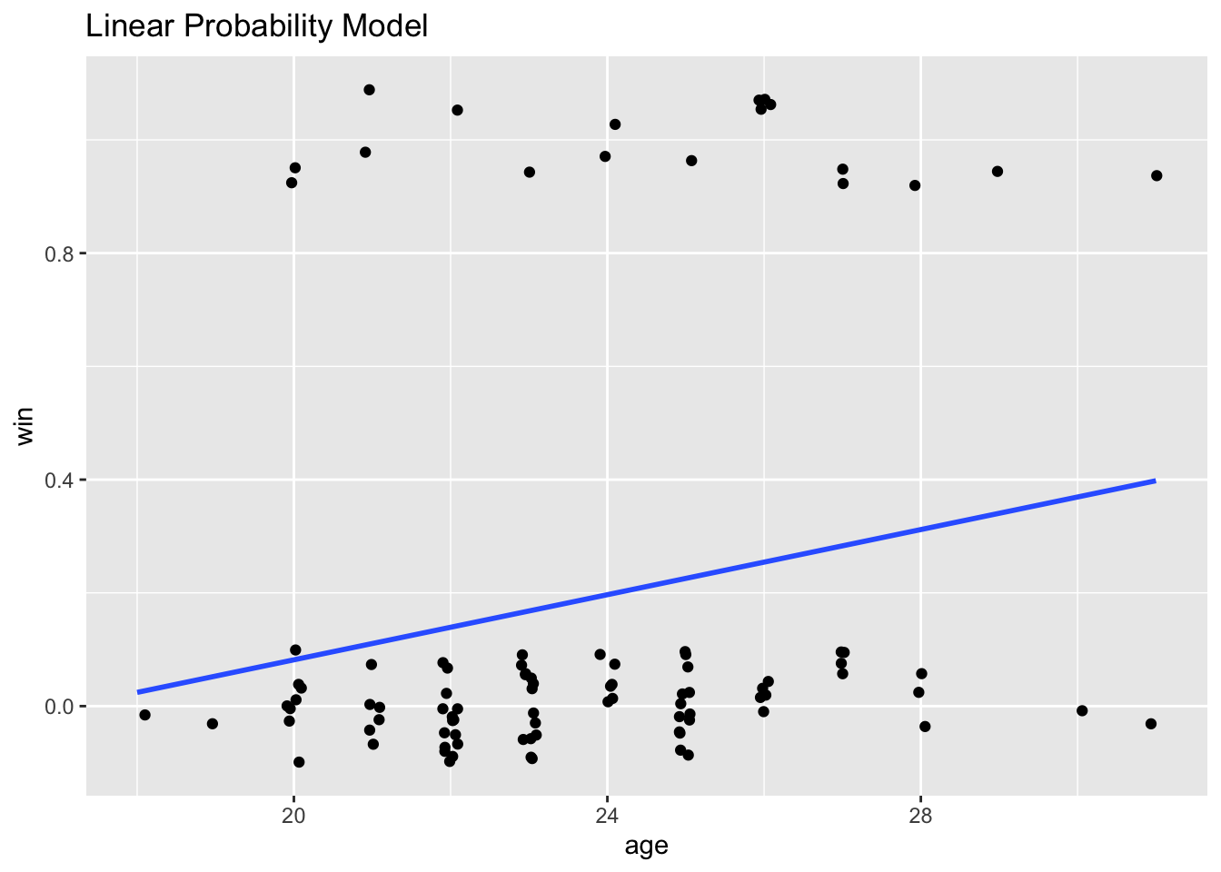
In classwork 5, we took the Love Island data set and estimated a linear probability model. The linear probability model uses a straight line to predict the probability of \(win = 1\):
\[\hat{p}(x) = \beta_0 + \beta_1 x\]
That can be useful for intuition, but it has a serious problem: it can easily predict probabilities below 0 or above 1, which are not valid.
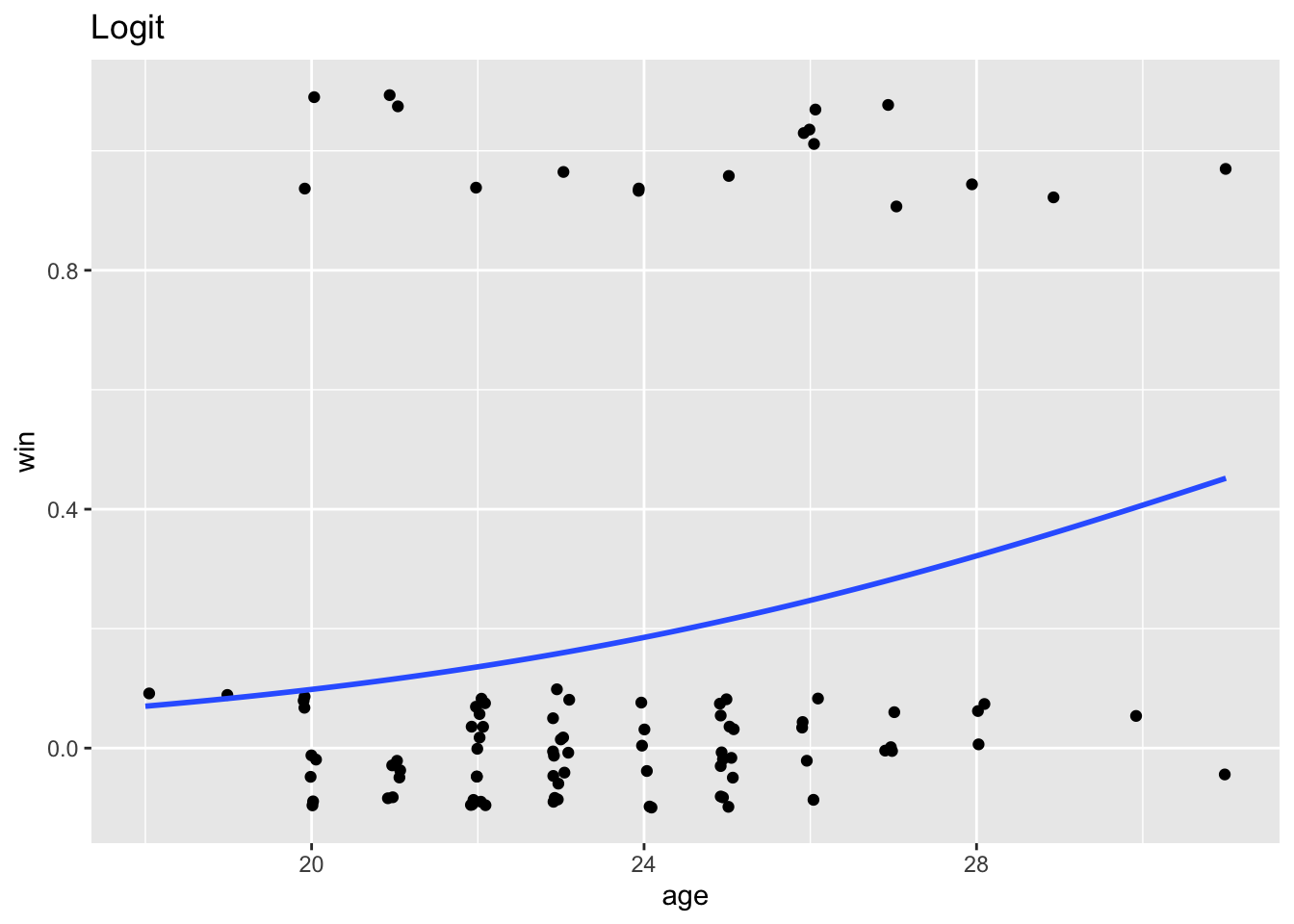
Here is the linear probability model and the logit side-by-side:
love %>%ggplot(aes(x = age, y = win)) +geom_jitter(width = .1, height = .1) +geom_smooth(method = lm, se = F) +labs(title ="Linear Probability Model")
love %>%ggplot(aes(x = age, y = win)) +geom_jitter(width = .1, height = .1) +geom_smooth(method ="glm", method.args =list(family ="binomial"), se = F) +labs(title ="Logit")
The logit curve is bounded by 0 and 1: it will never predict probabilities outside that range.
What is a Logit?
A logit model assumes the probability of success follows an S-shaped curve (linear in log odds, not in probability):
This function is called the logistic function. It has two big advantages:
It is bounded by 0 and 1
The effect of x on the probability of success can be large in the middle, and flatten out near probabilities of 0 and 1, which is realistic for many situations.
A rearrangement of the same model in terms of log odds:
Use them to compute predicted probabilities \(p_i\)
Plug them into the log-likelihood formula
Return the total log likelihood
Question 10
Fill in the blank so that the function outputs the log likelihood for a guess for \(\beta_0\) and \(\beta_1\).
# LL <- function(beta) {# b0 <- beta[1]# b1 <- beta[2]# # x <- love %>% pull(age)# y <- love %>% pull(win)# # p <- 1 / (1 + exp(-(b0 + b1 * x)))# # sum(___)# }
Step 2: Maximize the log likelihood
Question 11
Fill in the blank to get maxLik to estimate \(\beta_0\) and \(\beta_1\) for us in the logit.
# maxLik(# logLik = __,# start = c(0, 0)# )
Step 3: Interpreting the results
Question 12
What did you estimate \(\beta_0\) to be? What did you estimate \(\beta_1\) to be?
In a logit model, \(\beta_0\) is not the baseline probability and \(\beta_1\) is not the increase in probability when age increases by 1. Instead, they are in terms of log odds. To recover predicted probabilities, plug \(\beta_0\) and \(\beta_1\) back into the logistic function: