library(tidyverse)

fish <- read_csv("https://raw.githubusercontent.com/cobriant/teaching-datasets/refs/heads/main/fish.csv") %>%
  mutate(
    weekday = case_when(
      mon == 1 ~ "M",
      tues == 1 ~ "T",
      wed == 1 ~ "W",
      thurs == 1 ~ "R",
      .default = "F"
    ),
    weekday = factor(weekday, levels = c("M","T","W","R","F"))
  ) %>%
  select(price, quantity_sold, buyer_race, weekday, wind_speed, wave_height, day)

# 1) Visualize the distribution of the price of whiting.


# 2) Visualize the relationship between price (y-axis) and quantity sold (x-axis). Add a line of best fit with geom_smooth(method = lm).


# 3) Use a plot to answer the question, "Does price change based on the weekday?"


# 4) Use a plot to answer the question, "Does price change based on wind speed?"


# 5) Use a plot to answer the question, "Does price change based on wave height?" Add a line of best fit.


# 6) Visualize the relationship between price and buyer race.


# 7) Visualize the distribution of quantity_sold.


# 8) Use a plot to answer the question, "Do we see larger sales on some weekdays relative to others?"


# 9) Visualize the distribution of wind_speed.


# 10) Visualize the distribution of wave_height.


# 11) Use a plot to answer the question, "what is the relationship between wind speed and wave height?" Add a line of best fit.Ggplot2 and lm Review: Fulton Fish Market
In this classwork, we’ll review ggplot2 and lm by finishing our replication of Kathryn Graddy’s (2006) paper Markets: The Fulton Fish Market.
Use this cheat sheet as a reminder of the declarative programming tools we’ve learned. In this classwork, focus on the lower left decision tree for ggplot.
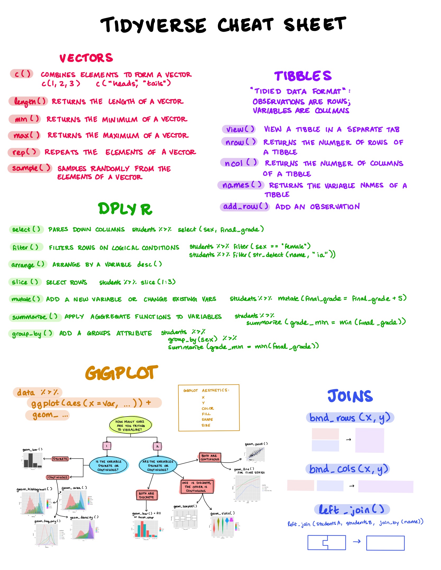
Part 1: Written Answers
Answer these questions by looking at the cheat sheet above:
List the six ggplot aesthetic mappings.
Which five geoms can you use to visualize the distribution of a single variable?
What’s the difference between geom_bar and geom_histogram?
What two geoms can you use to visualize the relationship between two variables when they’re both continuous?
What geom can you use to visualize the relationship between two variables when they’re both discrete?
Part 2: Ggplot Practice
Part 3: lm Practice
# 1) Use lm to show that asian buyers negotiate lower fish
# prices than white buyers, holding constant the weekday,
# wind speed, and wave height.

lm(price ~ ___ + weekday + wind_speed + wave_height, data = fish) %>%
  broom::tidy()

# Interpretation: Holding constant the day of the week,
# the wind speed, and the wave height, white buyers pay
# on average ___ cents per pound more for fish
# compared to asian buyers, which (is/is not
# statistically significant).

# 2. Use lm to verify that wind speed and wave height
# predict lower quantities of fish sold at the fish market,
# holding constant weekday and buyer race.


# Interpretation: When wind speed increases by 1 mile/hr,
# quantity sold decreases by ___, which (is/is not)
# statistically significant. When wave height increases
# by 1 unit, quantity sold decreases by ___, which
# (is/is not) statistically significant.
Now you can use the function ivreg to run an instrumental variables regression: the shifters wind_speed and wave_height are instruments for price: they show the effect of the shifting supply curve, tracing out the demand curve. The coefficient on log(price) is interpreted as the percent increase in the Y variable for a one percent increase in the X variable. That is, the coefficient on log(price) is the elasticity. An elasticity of -1 means that when price increases by 1%, quantity demanded decreases by 1%. An elasticity of -2 means that when price increases by 1%, quantity demanded decreases by 2%: the consumers are elastic. An elasticity of -0.5 means that when price increases by 1%, quantity demanded decreases by 0.5%: consumers are inelastic.
install.packages("ivreg")library(ivreg)
# 3) Use ivreg to estimate the price elasticity of demand
# for asian buyers and then white buyers.
fish %>%
filter(buyer_race == ___) %>%
ivreg(log(quantity_sold) ~ log(price) + weekday | wave_height + wind_speed + weekday, data = .) %>%
broom::tidy()
fish %>%
filter(buyer_race == ___) %>%
ivreg(log(quantity_sold) ~ log(price) + weekday | wave_height + wind_speed + weekday, data = .) %>%
broom::tidy()
# Interpretation:
# - When price increases by 1%, white buyers demand ___% fewer fish.
# - When price increases by 1%, asian buyers demand ___% fewer fish.
# - Perfectly inelastic buyers have a price elasticity of
# 0: when price increases by 1%, perfectly inelastic
#. buyers demand 0% fewer fish (their demand stays exactly
#. the same).
# - Perfectly elastic buyers have a price elasticity of
#. infinity: when price increases by 1%, perfectly elastic
#. buyers demand infinity % fewer fish (their demand goes
#. to 0).
# - Asian buyers respond more to price increases than
#. white buyers: their demand is more (elastic/inelastic).
#. This makes sense because asian buyers resell fish in
#. low-income neighborhoods or use it for products like
#. fishballs, so are very sensitive to price changes. But
#. white buyers are more likely to sell to high-end
#. restaurants or suburban retailers, so they have less
#. elastic demand because they can pass higher costs on to
#. their customers.Download this assignment
Here’s a link to download this assignment.