5 Nested Fixed Point

5.1 Introduction

In 1987, John Rust published a groundbreaking paper in Econometrica called Optimal Replacement of GMC Bus Engines: An Empirical Model of Harold Zurcher. In that paper, Rust laid out a solution method to estimate models of dynamic discrete choice called the Nested Fixed Point algorithm, and explained how it worked using a simple example about replacing bus engines. Now more than thirty years later, the Nested Fixed Point algorithm is still the most popular way to estimate DDC models.

John Rust in 2011

5.2 Harold Zurcher

John Rust was a professor of economics at the University of Wisconsin when he met Harold Zurcher. They were both riding the bus to work. Harold Zurcher was the superintendent of the Madison, Wisconsin Bus Company. Among other things, Zurcher kept tabs on each bus in the fleet and decided when a bus would receive regular maintenance versus when it needed an entire engine overhaul.

This struck Rust as a terrific example to explain what he was working on because Zurcher was an agent expertly playing the MDP “game”, making the binary decision about whether to replace a bus engine each period. A new engine drives smoothly, but as the engine accumulates mileage, it’s more likely to break down and require more and more expensive maintenance, which eventually makes it worth it to replace the engine entirely. An engine replacement is costly, but after the engine has been replaced, the bus runs as good as new.

5.3 The MDP

You learned in chapters 3 and 4 that Markov Decision Processes have an agent who selects among alternative actions that govern the Markov transition matrix going from one period to the next.

In this problem, Harold Zurcher is the agent. He can select among two alternatives: keep the engine or replace it. The state of the bus is a collection of many different variables: the status of each component, reports from bus drivers about how well the bus is driving, and even the number of open service bays Zurcher has available to perform maintenance on the bus. All of these are unobservable to us as econometricians however. There’s only one aspect of the bus state that you can observe: the engine mileage.

Harold Zurcher generously provided Rust with his logs: for each bus in his fleet, we know the engine mileage at the beginning of each month and the mileage when a bus received its first and second engine replacements, if its engine was replaced. The data spans 10 years for 104 different buses.

When Zurcher decides to replace the bus engine in a certain month, the Markov transition matrix looks like the matrix below (the mileage is reset back to 0 and remains there w.p. p0). Rust discretizes engine mileage into buckets of size 5000 miles, so “state 1” means that the engine has between 0 and 4999 miles on it; “state 2” means that the engine has between 5000 and 9999 miles on it, etc. There are 90 states in total, and the 90th state is absorbing just like in the lemon tree example. So the transition probability matrices are 90x90 and look like this:

\[\begin{equation} T_{replace} = \begin{bmatrix} p0 & p1 & p2 & 0 & 0 & 0 & ...\\ p0 & p1 & p2 & 0 & 0 & 0 & ...\\ p0 & p1 & p2 & 0 & 0 & 0 & ...\\ ... \end{bmatrix} \end{equation}\]

Whereas when Zurcher decides to keep the bus engine, this transition matrix governs the mileage in the next month. This should remind you of “watering” your lemon tree with p0 on the diagonal:

\[\begin{equation} T_{keep} = \begin{bmatrix} p0 & p1 & p2 & 0 & 0 & 0 & ...\\ 0 & p0 & p1 & p2 & 0 & 0 & ...\\ 0 & 0 & p0 & p1 & p2 & 0 & ...\\ ... \end{bmatrix} \end{equation}\]

Rust used the data to estimate p0, p1, and p2. Here are the probabilities he calculated:

p0 <- .3489
p1 <- .6394
p2 <- 1 - p0 - p1

Exercise 1: In R, create the 90x90 transition matrix for keeping the engine and call it transition. Make sure to make the 90th state absorbing. Check that the sum of each row is 1: all(rowSums(transition) == 1).

5.4 Unobservables

Here I load the data on bus mileage and Zurcher’s decision to replace the engine. Engines were replaced 59 times in the 10 year period for these 104 buses. The plot below shows the mileage when the engine was replaced: no engine was replaced that had a mileage less than bucket 25 (120,000 miles), but after mileage bucket 25, there’s large variation. Clearly, to make his decision about engine replacement, Zurcher was thinking about more than just mileage.

library(tidyverse)

bus <- read_csv("https://raw.githubusercontent.com/cobriant/dplyrmurdermystery/master/bus.csv")

bus %>%
  filter(replace == TRUE) %>%
  ggplot(aes(x = mileage)) +
    geom_histogram() +
    ggtitle("Mileage at Replacement")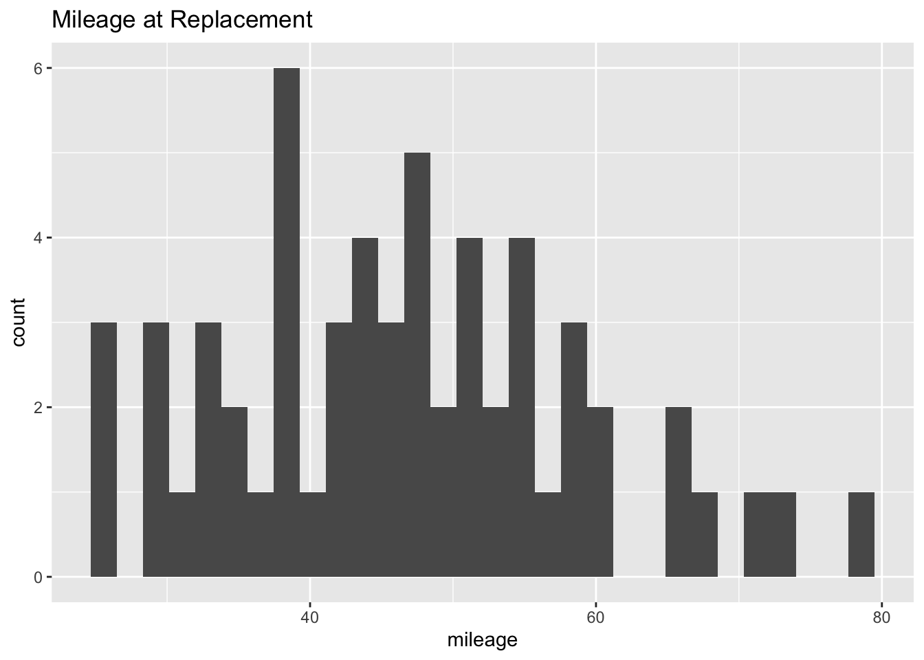

5.4.1 Conditional Independence Assumption

The major assumption for the validity of our estimation strategy is called conditional independence. It is similar to the OLS exogeneity assumption, but not quite as restrictive.

Let the bus mileage at time t be \(x_t\) and let the unobserved term be \(\varepsilon_t\) (impact of a component failure, positive or negative report from the driver, or bus breakdown).

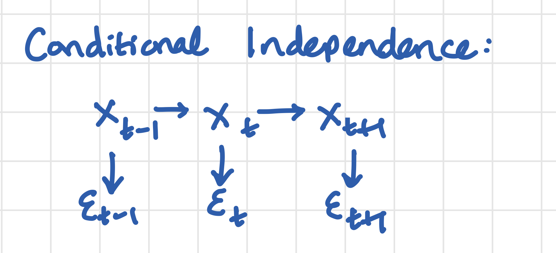
You don’t need to assume that \(x_t\) and \(\varepsilon_t\) are independent random variables: of course if the bus has more miles on it, it has a higher risk of having a component fail or breaking down entirely. We also allow for \(x_t\) to be autocorrelated: it will increase by 0, 1, or 2 mileage buckets each period as long as the engine is not replaced, so it will be a highly autocorrelated series.

But we need to assume \(\varepsilon\) is only autocorrelated through the way it correlates with \(x\). So if a component fails in one period, the issue will be fixed when the bus gets maintenance, and it does not mean another component is more likely to fail, except through the fact that the bus is getting worn down by mileage.

The consequence of the conditional independence assumption is that \(future\_value\), the expected future value of having just been in a state, does not depend on \(\varepsilon\). Instead, the value of leaving the state can be completely summed up by a function of \(x_t\), the mileage bucket, and not on \(\varepsilon_t\). Without the conditional independence assumption, we would have to include \(\varepsilon\) in the state because the expected future value of having a bus that was just in mileage bucket 30 with a large negative value for \(\varepsilon\) would be much less than having a bus in mileage bucket 30 with a positive value for \(\varepsilon\). Conditional independence is perhaps restrictive, but it allows the problem to be tractable.

I think what’s most compelling about this paper is that John Rust only saw a piece of the picture: the mileage readings and replacement decision. As the econometricians, we don’t know when a part was failing, or when a driver was reporting to Zurcher that the bus wasn’t working as well, or even when a bus broke down. But using only the piece of the picture about mileage, we can fit a model that explains the MDP Zurcher was playing.

5.4.2 What DDC lets you do

The NFXP algorithm will let us parameterize the MDP. In particular, two important parameters characterize the MDP: costs related to replacing the engine, and then if you want to avoid replacing the engine, the costs related to maintaining the old one. I’ll call these parameters theta[1] and theta[2].

theta[2]: Replacing the engine is expensive. You have to buy a new engine, and then there are labor costs associated with installing it.

theta[1]: If you don’t replace the engine, each month you may have to fix a couple components and do a host of other regular maintenance on the bus to keep it in good working order. These costs go into theta[1], but there are also other costs related to keeping an old engine: costs related to the possibility that the bus breaks down, needs towing, and there will be a loss of rider goodwill. Maintenance costs also increase as the bus accumulates more mileage, so we’ll actually have maintenance costs be theta[1] * .001 * (1:90), which assumes maintenance costs increase linearly with mileage bucket, where theta[1] is the slope. The .001 scales the number so it has the same magnitude as theta[2], which will help us during the numerical optimization part.

Harold Zurcher could theoretically estimate theta[2] for us, but he might have trouble estimating theta[1] well: a lot of variables go into it. DDC lets us look at Zurcher’s behavior and use that to estimate the ratio between theta[1] and theta[2]. Then we can use Zurcher’s estimate of theta[2] to find out what theta[1] is, quantifying a previously unquantifiable average cost.

5.4.3 Key Terms and Notation

Symbol	Meaning
\(x_t\)	Mileage on the odometer for a bus in a certain month
\(\varepsilon_t\)	Unobservable part of the state: anything about the bus that is not mileage that effects Zurcher’s decision to replace the engine or not. So this includes status of various bus components, reports from bus drivers about how well the bus is running, and the number of available service bays Zurcher has at the time.
\(\theta_1\)	The point of this whole algorithm is to be able to estimate two values \(\theta_1\) and \(\theta_2\), that describe the data generating process. \(\theta_1\) is the replacement cost: any expense related to purchasing and installing a new bus engine.
\(\theta_2\)	This is the parameter describing average regular maintenance costs of buses. In particular, maintenance costs are the 90x1 matrix \(\theta_2 \times .001 \times 1:90\). The .001 scales the number so it has the same magnitude of \(\theta_1\), which will help us during the numerical optimization part. The 1:90 means we assume costs increase linearly with mileage: a bus in mileage bucket 1 has expected maintenance costs of \(\theta_2 \times .001\), and a bus in mileage bucket 2 has expected maintenance costs of \(\theta_2 \times .001 \times 2\).

5.5 Inner Loop

The inner loop should feel familiar based on the value function iteration we did in chapter 4. There are 4 parts to the inner loop, and each of them are 90x1 matrices (except for value_replace): value, value_replace, value_keep, and future_value.

5.5.1 value

value is a 90x1 matrix that tells you how valuable it is on average to be in each state (mileage bucket) assuming you behave optimally. In chapter 4, we used pmax: value <- pmax(value_keep, value_replace). In this chapter, I’ll make a small change: the optimization algorithm will struggle with functions like max() and pmax() because they are non-differentiable (too pointy). So instead of using pmax(), I’ll use a smooth, differentiable approximation to pmax(), the log-sum-exp operator.

logsumexp <- function(x, y) {
    log(exp(x) + exp(y))
}

# When x and y are close, logsumexp is a rough approximation for the maximum:
logsumexp(1, 2)

[1] 2.313262

# But when x and y are further apart, logsumexp does a better job:
logsumexp(1, 10)

[1] 10.00012

There’s one more adjustment to logsumexp() that we should make: when x is large in absolute value, exp(x) will overflow and it will return Inf or -Inf. To see for yourself: run exp(1000) in R. So to avoid overflow, we can do something called the “log-sum-exp” trick, that is to subtract the maximum before doing the operation and then add it back in afterward.

logsumexp <- function(x, y) {
    max <- max(x, y)
    max + log(exp(x - max) + exp(y - max))
}

Exercise 2: Verify that the log-sum-exp trick is valid by plugging in some different numbers for x and y and showing that log(exp(x) + exp(y)) == log(exp(x - max(x, y)) + exp(y - max(x, y))) + max(x, y).

To summarize, value will not be pmax(value_keep, value_replace), but it will instead be:

value <- logsumexp(value_keep, value_replace)

5.5.2 value_replace

value_replace is a scalar that tells us how expensive it is to replace the engine and then behave optimally thereafter. If we let the cost of replacing an engine be theta[2], then the value of replacing an engine would be - theta[2] plus the discounted future value of having been in state 1, because the mileage gets reset after engine replacement.

value_replace <- - theta[2] + beta * future_value[1]

5.5.3 value_keep

value_keep is another 90x1 matrix that tells us how expensive we should expect it to be if, for each period, we kept the current engine instead of replacing it, then behaved optimally after that. So value_keep will be the maintenance cost of having the older engine - theta[1] * .01 * 1:90 plus the discounted future value of having been in that state:

value_keep <- - theta[1] * .001 * 1:90 + beta * future_value

5.5.4 future_value

The final piece is future_value, another 90x1 matrix. Just like in Chapter 4, this is the expected future value having just been in the state. So it’s the probability you’ll stay in the same state next period (p0) times the value of being in the same state, plus the probability you’ll move to the next state next period (p1) times the value of being in that state, plus the probability you’ll move two states up next period (p2) times the value of being in that state.

\[future\_value[1] = p0 \ v[1] + p1 \ v[2] + p2 \ v[3] \tag{5.1}\]

And future_value[2] is this:

\[future\_value[2] = p0 \ v[2] + p1 \ v[3] + p2 \ v[4] \tag{5.2}\]

So the formula to find EV is this: \(future\_value = transition \times value\).

future_value <- transition %*% value

Exercise 3: Write a function inner_loop that takes a vector of length 2 theta and does value function iteration until value converges (value and value_next are within 0.1 of each other). The function should output the matrix value. Show that when maintenance costs and replacement costs are both 5: inner_loop(c(5, 5)) returns values between 47 and 52. Use beta = 0.9999.

5.6 Outer Loop

The inner loop does value iteration so that given a guess for theta, we can find the value function. The outer loop takes the value function, uses it to find choice probabilities (remember chapter 1 on logits?), which we can use to find the likelihood of observing Zurcher’s data. Then we can use maxLik to search all possible values for theta to find the values that maximize the likelihood function.

Let’s take it step-by-step:

1. Use the value function from inner_loop() to find the logit choice probabilities
1. Use the choice probabilities to find the likelihood
1. Use maxLik to find the values for theta that maximize the likelihood

5.6.1 Value function to choice probabilitiy

We’ve just defined the inner loop: given a guess for theta, we can find value through the method of value iteration. We can use value to calculate future_value, value_keep, and value_replace.

The logit choice probability is the probability that Zurcher keeps the engine instead of replacing it given its mileage. Recall from chapter 1 that if \(\varepsilon\) has the extreme value distribution, we can use the logit choice probability: \(Prob(big \ mac) = F(V_{diff}) = \frac{exp(V_{diff})}{1 + exp(V_{diff})}\). So the logit choice probability for keeping the engine instead of replacing it is:

\[p_{keep} = \frac{exp(v_{keep} - v_{replace})}{1 + exp(v_{keep} - v_{replace})} \tag{5.3}\]

Exercise 4: Show that Equation 5.3 can be reorganized to \(p_{keep} = \frac{exp(v_{keep})}{exp(v_{keep}) + exp(v_{replace})}\)

Exercise 5: To avoid overflow with exp(), we’ll subtract the maximum of future_value. Show that this formula is equivalent to the one from exercise 4: \(p_{keep} = \frac{exp(v_{keep} - max(future\_value))}{exp(v_{keep} - max(future\_value)) + exp(v_{replace} - max(future\_value))}\).

So the formula we’ll use for p_keep is:

p_keep <- function(theta, future_value) {
  exp_vk <- exp(-theta[1] * .001 * (1:90) + beta * future_value - max(future_value))
  exp_vr <- exp(-theta[2] + beta * future_value[1] - max(future_value))
  exp_vk / (exp_vk + exp_vr)
}

5.6.2 Choice probability to likelihood

In Chapter 2 (2.3 Logit Estimation), we took data and a choice probability and calculated the log likelihood of observing that data. In this section, I will follow the same pattern.

I wanted to get it into a format that would make the computation of the (partial log) likelihood of the data as simple as possible, so for each mileage bucket (1-90), I counted the number of times n we were in that state and chose whether or not to replace the engine. So reading the first two rows goes like this: in total, Zurcher had buses in mileage bucket 1 286 times, and never once in those 286 times did he decide to replace the engine.

rust <- read_csv("https://raw.githubusercontent.com/cobriant/dplyrmurdermystery/master/rust.csv")

Rows: 180 Columns: 3
── Column specification ────────────────────────────────────────────────────────
Delimiter: ","
dbl (2): mileage, n
lgl (1): replace

ℹ Use `spec()` to retrieve the full column specification for this data.
ℹ Specify the column types or set `show_col_types = FALSE` to quiet this message.

rust

# A tibble: 180 × 3
   replace mileage     n
   <lgl>     <dbl> <dbl>
 1 FALSE         1   286
 2 TRUE          1     0
 3 FALSE         2   215
 4 TRUE          2     0
 5 FALSE         3   221
 6 TRUE          3     0
 7 FALSE         4   263
 8 TRUE          4     0
 9 FALSE         5   255
10 TRUE          5     0
# … with 170 more rows

Exercise 6: Assume we know the logit choice probability, that is, the probability Zurcher will keep the bus engine versus replace it given the bus is in a certain mileage bucket. Write a function log_lik that takes that choice probability (the probability you keep the engine is a 90x1 matrix p_keep) and returns a ~~single number~~ vector of length 90 that is the partial log likelihood of observing the data.

Hint for Exercise 6: Suppose we’re doing a simpler problem where there are only 3 mileage buckets and we’ve estimated that p_keep = (.8, .6, .2). Suppose also that we are in mileage bucket 1 286 times and that we never replace the engine. Then we’re in mileage bucket 2 200 times, replacing the engine 100 times and not replacing 100 times. Then we’re in mileage bucket 3 50 times, replacing the engine all 50 times. Then the partial log likelihood of observing this data would be:

# 286 * .8: We kept the engine 286 times in bucket 1, where we had a probability of keeping it of .8
# 100 * .6: We kept the engine 100 times in bucket 2, where we had a probability of keeping it of .6
# 100 * .4: we replaced the engine 100 times in bucket 2, where we had a probability of replacing it of 1 - .6 = .4
# 50 * .8: We replaced the engine 50 times when we were in bucket 3, when we had a probability of replacing it of 1 - .2 = .8.
c(286 * log(.8), 100 * log(.6) + 100 * log(.4), 50 * log(.8))

[1]  -63.81906 -142.71164  -11.15718

5.6.3 maxLik

The outer loop guesses theta, finds value through the inner loop, and finally calculates p_keep to calculate log_lik(p_keep). That’s a measure of the likelihood that theta are the true maintenance and replacement costs of bus engines.

The outer loop then searches different values for theta until it finds values that maximize log_lik(p_keep). We’ll use maxLik::maxBHHH to do that optimization step for us. Here’s the algorithm. It takes about 30 seconds to run on my computer, so do not be surprised if it doesn’t execute immediately on yours. You’ll of course need to include transition, inner_loop, and log_lik.

library(maxLik)

beta <- .9999
p0 <- .3489
p1 <- .6394
p2 <- 1 - p0 - p1

# transition <- ___

logsumexp <- function(x, y) {
  max <- max(x, y)
  max + log(exp(x - max) + exp(y - max))
}

# inner_loop <- function(theta) {
# 
# }

pk <- function(theta, value) {
  future_value <- transition %*% value
  value_keep <- - theta[1] * .001 * (1:90) + beta * future_value
  value_replace <- - theta[2] + beta * future_value[1]
  exp_vk <- exp(value_keep - max(future_value))
  exp_vr <- exp(value_replace - max(future_value))
  return(exp_vk / (exp_vk + exp_vr))
}

# log_lik <- function(p_keep) {
#   
# }

likelihood <- function(theta) {
    value <- inner_loop(theta)

    pk(theta, value) %>%
      log_lik()
}

results <- maxLik::maxBHHH(likelihood, start = c(1, 9))
summary(results)

Exercise 7: Do your results get close to the results from the original paper (hint: look at page 24 under (bus) Groups 1, 2, 3, and 4 and \(\beta\) = .9999)? Include an R script compiled to html to show your NFXP implementation and the final result.

5.7 References

Rust (1987) Optimal Replacement of GMC Bus Engines: An Empirical Model of Harold Zurcher.