A discrete choice is a choice among distinct alternatives. The choice could be binary (“buy it” or “don’t”), or there could be many alternatives (“buy nothing”, “buy a hamburger”, “buy 2 hamburgers”, “buy spaghetti”, etc). In this workbook, I’ll make our lives a lot simpler by focusing only on binary choices: the agent can choose option A or option B, they can’t choose both and they can’t choose neither.
Discrete choices are in constrast to continuous choices, measured on a continuous scale (how many ounces of spaghetti would you like?). A variable that’s discrete is counted while a variable that’s continuous is measured.
If you look through the previous book on OLS, you’ll notice that while discrete variables often entered into our models as explanatory variables, our dependent variables were always continuous:
Wage or earnings
Consumption
Life expectancy
GPA
We never modeled a discrete choice because OLS isn’t the best tool for the job. In this chapter, you’ll learn about a better alternative for modeling discrete choices: a logistic regression, or logit for short. The logit can’t be estimated using OLS because the model is not linear in parameters, so you’ll learn about a new estimation strategy in the next chapter called “maximum likelihood estimation”.
1.2 Notation
In this chapter, I use four greek letters you may or may not have seen recently:
symbol
pronounciation
\(\alpha\)
alpha
\(\beta\)
beta
\(\varepsilon\)
epsilon
\(\gamma\)
gamma
I also refer to the exponential function with \(exp()\): \(exp(x)\) means the same thing as \(e^x\) where \(e\) refers to euler’s number 2.718281…
1.3 Logit
As economists, we usually think the decisionmaker selects the alternative that provides the most utility. So if option A is a big mac and option B is a chicken sandwich, they will choose a big mac if: \[\text{Utility}_i^{big \ mac} > \text{Utility}_i^{chicken}\]
The first major assumption for the logit to be valid comes in here: utility functions must be additively separable: that is, utility is an observable part \(V\) added to an unobservable part \(\varepsilon\):
The observable part \(V\) is some linear function of observables (explanatory variables). Suppose age and gender are predictive of the utility people get from big macs and from chicken sandwiches: \[V_i^{big \ mac} = \alpha_0 + \alpha_1 age_i + \alpha_2 male_i\]\[V_i^{chicken} = \gamma_0 + \gamma_1 age_i + \gamma_2 male_i\]
Exercise 1: Suppose in the equations above, you have that \(\alpha_0 = 1\), \(\alpha_1 = -.1\), \(\alpha_2 = .5\), \(\gamma_0 = -1\), \(\gamma_1 = .2\), and \(\gamma_2 = -.3\). Find \(V_i^{big \ mac}\) and \(V_i^{chicken}\) for the average 20 year old male and the average 50 year old female. If \(\varepsilon_i^{big \ mac} = 0\) and \(\varepsilon_i^{chicken} = 0\) for a 20 year old male, should you expect that he will buy a big mac or a chicken sandwich?
The logit doesn’t help us to estimate a person’s \(V_i^{big \ mac}\) or \(V_i^{chicken}\). What it does help us to estimate is the person’s \(V_i^{diff} = V_i^{big \ mac} - V_i^{chicken}\), and then it helps us to estimate the probability that someone with certain values for the explanatory variables will make a certain decision. So we don’t know how much utility someone gets from an option, but that number doesn’t matter. It’s the relative utility they get from different options that impacts their decision.
So the agent will buy a big mac only if the difference between their shocks to \(\varepsilon\) in favor of big macs exceed \(V_i^{diff}\) in favor of chicken. Multiplying by -1 for convenience later, they’ll buy a big mac if:
If the distribution of \(\varepsilon_i^{diff} = \varepsilon_i^{chicken} - \varepsilon_i^{big \ mac}\) is known, and if we also know \(V_i^{diff} = V_i^{big \ mac} - V_i^{chicken}\), then we can calculate this choice probability. If we think that \(\varepsilon\) is distributed normally, then because the sum of two normals is normal, the difference between two normals is also normal. In that case, you’ll use a probit.
We’ll instead use a logit, which assumes that \(\varepsilon\) has the extreme value distribution. If \(\varepsilon_i\) is distributed extreme value, that implies that the difference in two \(\varepsilon_i\)’s has the logistic distribution (hence the name “logistic regression” or “logit” for short). Deciding between using a probit or a logit is generally inconsequential according to Kenneth Train’s excellent textbook on Discrete Choice:
Using the extreme value distribution for the errors (and hence the logistic distribution for the error differences) is nearly the same as assuming the errors are independently normal. The extreme value distribution gives slightly fatter tails than a normal, which means that it allows for slightly more aberrant behavior than the normal. Usually, however, the difference between extreme value and independent normal errors is indistinguishable empirically. Train (2009)
The CDF (cumulative distribution function) for the logistic distribution is this:
# Recall that pnorm() works like this:# If X is distributed N(0, 1), the probability that X is less than 0:pnorm(0)
[1] 0.5
# The same way, plogis() works like this:# If epsilon_diff has the logistic distribution, the# probability that epsilon_diff is less than -2:plogis(-2)
[1] 0.1192029
# And if a 20 year old male has a V_diff of 1 in favor of big macs,# the predicted probability he will buy a big mac is:plogis(1)
[1] 0.7310586
Exercise 2: If you estimate a person has a \(V^{diff} = -1\) in favor of big macs, what is the predicted probability they will buy a big mac (assuming \(\varepsilon\) has the extreme value distribution)?
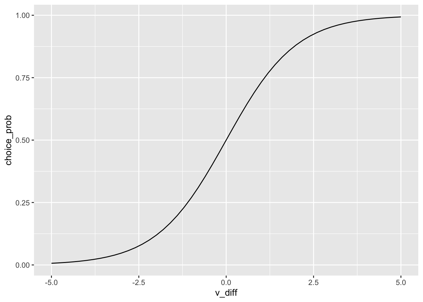
The logit model traces out the choice probabilitiy for all people on the \(V^{diff}\) horizontal line:
library(tidyverse)
tibble(v_diff =seq(-5, 5, by = .2),choice_prob =plogis(v_diff)) %>%ggplot(aes(x = v_diff, y = choice_prob)) +geom_line()
The logit choice probability is the logistic CDF evaluated at \(V_{diff}\):
\[Prob(big \ mac) = \frac{exp(\beta_0 + \beta_1 age + \beta_2 male)}{1 + exp(\beta_0 + \beta_1 age + \beta_2 male)} \tag{1.1}\]
This is the logit. Notice: it is not linear in parameters, so you can’t use OLS to estimate it.
But what about a much simpler model of the choice probability \(Prob(big \ mac)\); one that can be estimated using OLS:
\[Prob(big \ mac) = \beta_0 + \beta_1 age + \beta_2 male + \varepsilon\]
This is called the linear probability model. I’ll discuss it, along with its shortcomings, in the next section. Then I’ll finish the chapter discussing a few more aspects of the logit.
1.4 Linear Probability Model
Consider using OLS to fit this model:
\[Prob(big \ mac) = \beta_0 + \beta_1 age + \beta_2 male + \varepsilon\]
using data that looks like this:
Big Mac (1) or Chicken Sandwich (0)
Age
Male (1) or Female (0)
1
58
1
0
33
0
1
17
0
0
23
1
1
59
1
Interpreting this data: the first person is a 58 year old male who buys a big mac. The second person is a 33 year old female who buys a chicken sandwich.
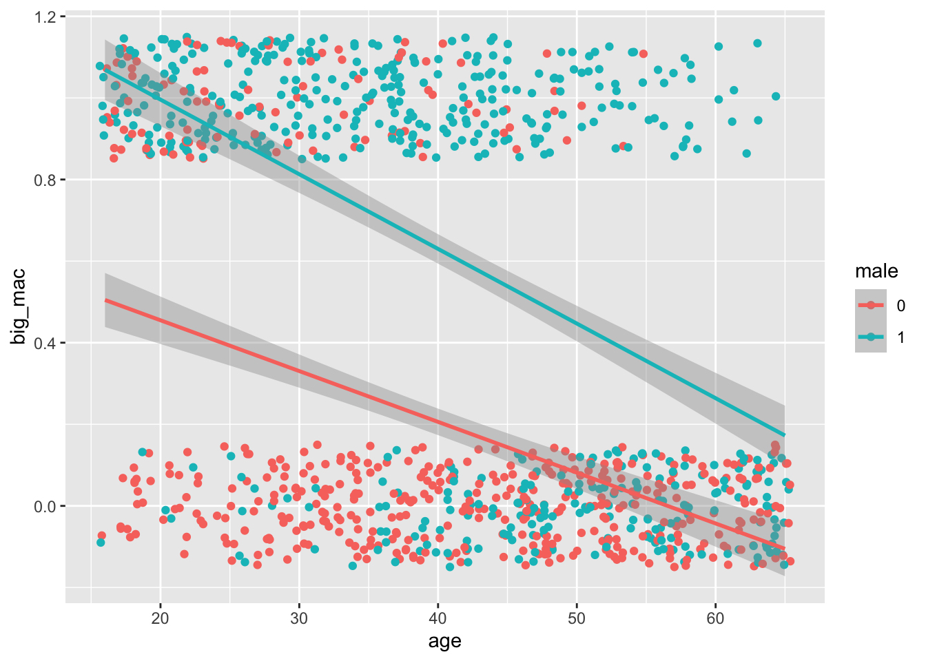
One option would be to use OLS. Here I load an artificial dataset and visualize this model. Notice I use geom_jitter() instead of geom_point() because the overplotting would make the plot very hard to understand:
Code
library(tidyverse)set.seed(1234)# Here I generate some artificial logit data:data <-tibble(# Let ages be between 16 and 65age =sample(16:65, replace = T, size =1000), male =sample(0:1, replace = T, size =1000),# The (observable) value someone gets from a big mac depends on their age and sex:v =2- .1* age +2.8* male,# The probability they buy a big mac depends on v according to the logit:prob_big_mac =exp(v) / (1+exp(v)), # They buy a big mac with the probability prob_big_mac.big_mac =rbinom(n =1000, size =1, prob = prob_big_mac)) %>%mutate(male =as.factor(male))
data %>%ggplot(aes(x = age, y = big_mac, color = male)) +geom_jitter(height = .15) +geom_smooth(method = lm)
`geom_smooth()` using formula 'y ~ x'
lm(big_mac ~ age + male, data = data) %>% broom::tidy(conf.int =TRUE)
This is called a linear probability model because it’s linear in parameters and you can interpret the fitted values for big_mac as the probability that someone will buy a big mac over a chicken sandwich given their age and gender.
Exercise 3: Interpret the estimates for this linear probability model. In particular, what’s the estimated probability that a 16 year old male will buy a big mac? And what’s the estimated probability a 50 year old female will buy a big mac?
There are two big problems with this linear probability model:
Estimated probabilities can easily be less than 0 or greater than 1, which makes no sense for probabilities. Nothing about OLS guarantees that the fitted values are reasonable numbers for probabilities.
We’ve assumed the relationship between the explanatory variables and the probability someone buys a big mac over a chicken sandwich is linear, but this might not reflect reality. We’d probably prefer a model that lets marginal effects change: for example, maybe going from age 15 to age 25 doesn’t change the probability you’ll buy a big mac very much, but going from age 45 to 55 creates a much larger behavioral change.
1.5 Logit to the rescue
Guess what: the logit solves both these problems: instead of \(Prob(\ big \ mac_i)\) on the left hand side, we’ll have the log odds of buying a big mac on the left hand side. Odds are just the probability you do the thing divided by the probability you don’t.
Exercise 4: Show that if you take the model above and solve for \(Prob(big \ mac)\), you’ll get that: \[Prob(big \ mac)_i = \frac{exp(\beta_0 + \beta_1 age_i + \beta_2 male_i)}{1 + exp(\beta_0 + \beta_1 age_i + \beta_2 male_i)}\] Which is exactly the way I defined the logit in Equation 1.1.
Exercise 5: A logit will never predict a probability outside of the \((0, 1)\) range. Show that this is true using the formula from Equation 1.1. In particular, consider what \(Prob(big \ mac)_i\) will be if \(\beta_0 + \beta_1 age_i + \beta_2 male_i\) is very large, like 1,000,000, or very negative, like -1,000,000.
1.5.1 Logits predict varying marginal effects
Take \(\beta_0 = -2\) and \(\beta_1 = .05\) for a logit with just one explanatory variable. We can take the formula \(Prob(option \ A)_i = \frac{exp(\beta_0 + \beta_1 x_i)}{1 + exp(\beta_0 + \beta_1 x_i)}\) and plot \(Prob(option \ A)\) on the y-axis against the explanatory variable x on the x-axis:
The plot above shows that marginal effects for logits can vary. Here, they start small, increase, and then decrease (I’m looking at the slope of the curve above). That is, going from x = 15 to 25 creates a small increase in the probability you’ll take option A over option B, but not as much as the behavioral change going from x = 40 to 50. And by the time x = 90 or 100, the marginal impact of x on the probability you’ll take option A is small again (perhaps because everyone possibly interested in taking option A is already taking it).
1.6 Logit Coefficient Interpretation
To interpret the coefficients \(\hat{\beta_0}\) and \(\hat{\beta_1}\) for a logit, consider the model again:
\(\hat{\beta_0}\) is the estimated log odds of “a success” given x = 0. \(\hat{\beta_1}\) is the estimated increase in the log odds of a success when x increases by 1 unit.
I’ll use glm() to fit the logit for the big mac example using artificial data. I’ll discuss a little of what’s going on behind the scenes to fit this model in the next chapter on Maximum Likelihood Estimation.
glm(big_mac ~ age + male, data = data, family ="binomial") %>% broom::tidy(conf.int =TRUE)
Exercise 6: Interpret these estimates by answering: what is my estimate for the probability that a 20 year old male will get a big mac? And what about a 50 year old female?
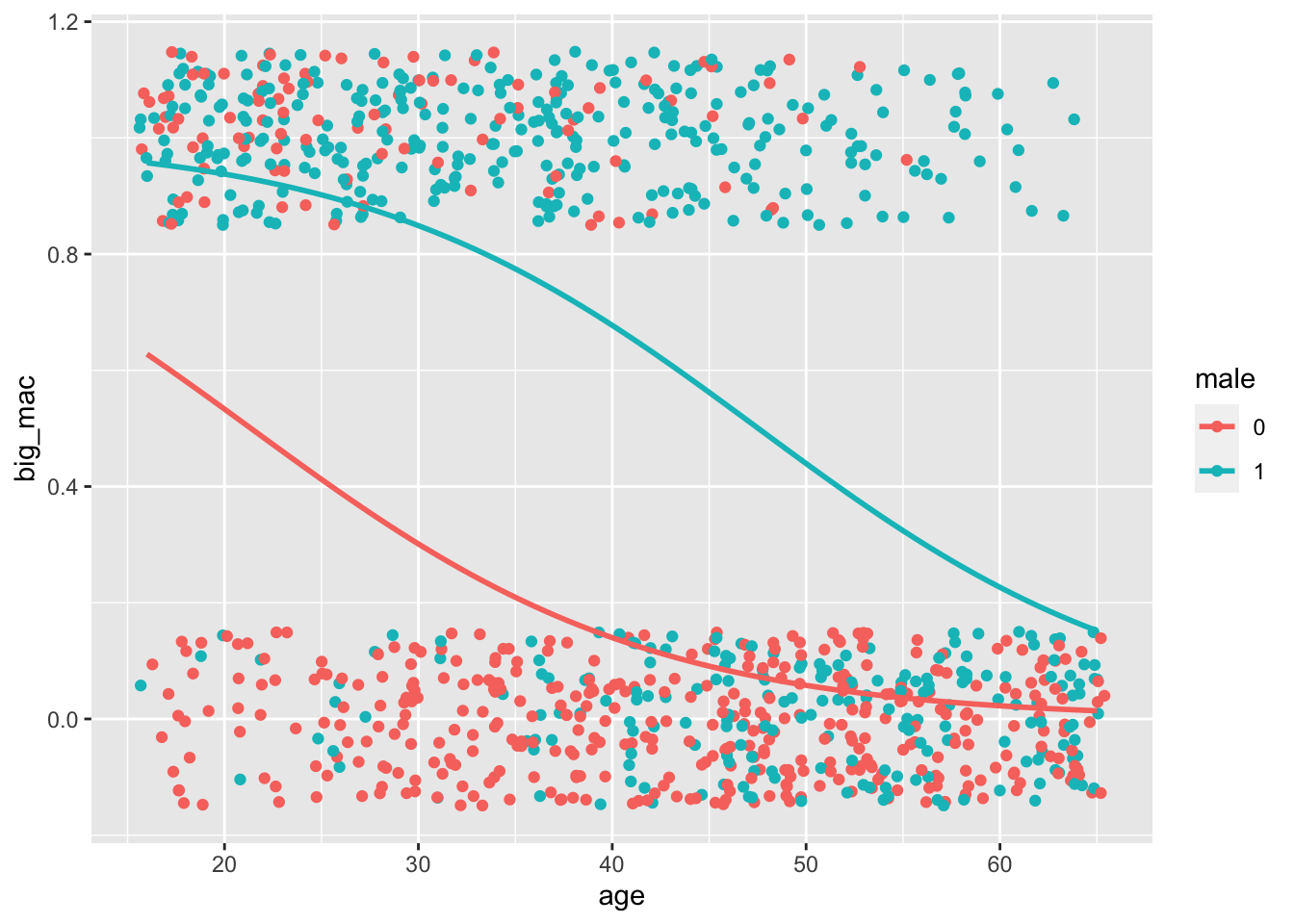
Finally, I’ll visualize the logit I just estimated:
data %>%ggplot(aes(x = age, y = big_mac, color = male)) +geom_jitter(height = .15) +stat_smooth(method ="glm", se =FALSE, method.args =list(family = binomial))
`geom_smooth()` using formula 'y ~ x'
1.7 Programming Exercises
Exercise 7: Go to Project Euler and create an account. Doing this will let you check your answer to the problems you’re about to do. Then go to Archives and solve problem 1: If we list all the natural numbers below 10 that are multiples of 3 or 5, we get 3, 5, 6 and 9. The sum of these multiples is 23. Find the sum of all the multiples of 3 or 5 below 1000. If you’re having trouble getting started, take a look at the programming tools section in the back of this workbook.
1.8 References
Dougherty (2016) Chapter 10: Binary Choice and Limited Dependent Variable Models, and Maximum Likelihood Estimation