10 IV for Simultaneous Equations
10.1 Introduction
In your Principles of Micro or Macro classes, you probably learned about the “Marshallian Cross” model of the determination of market prices. The demand curve slopes down and the supply curve slopes up, and the equilibrium price and quantity exchanged are at the intersection of those two curves. So if you had data on prices and quantities exchanged and you ran a regression like this one: lm(q ~ p), would you be estimating the supply curve or the demand curve? The answer is neither, because of simultaneous equation bias.
10.2 Biases We’ve Studied Thus Far
Simultaneous equation bias is something new, bus it’s still based on a failure of exogeneity. Recall, these are the biases we’ve learned about thus far:
Omitted variable bias. Selection bias is a type of OVB where the omitted variable is someone’s propensity to select in to treatment. OVB may bias an estimate up or down depending on the relationships between x and o, as well as y and o.
Measurement error. When X is measured with error, we’ll estimate an effect of X on Y that is attenuated (closer to 0 than the true value).
Lagged dependent variable models:
lm(y ~ lag(y)). When \(u_t\) is autocorrelated, we also get inconsistency for this model.
The root issue for all these cases is that exogeneity was violated: \(E[u_i | X] \neq 0\). The same is true for the new source of bias for this chapter:
- Simultaneity Bias: when data is generated by the interaction of two or more equations simultaneously.
To see how exogeneity would be violated in the market described in the video above, suppose we’re trying to estimate the demand curve \(q_i^d = \alpha_0 + \alpha_1 p_i + u_i\) where \(u_i\) refers to demand shifters like advertising. Exogeneity means:
\(E[u_i | P] = 0\)
That is, if you were told that in one location, the price was high, and in the other location, the price was low, you would have no idea which location may have had the advertising campaign. This is not a valid assumption, because advertising and price tend to be closely linked through many different channels: this is the simultaneity.
10.3 IV to the Rescue
In the previous chapter, we learned how an exogeneous instrument Z can help us estimate the causal effect of X on Y even when the data generating process suffers from OVB.
In the same way, an exogenous instrument Z can help us estimate the slope of the supply (or demand) curve even when the DGP is from two simultaneous equations.
10.4 Example 1: Market for Coffee
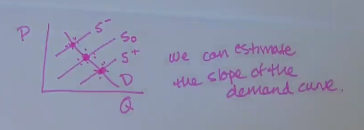
In this example, we’ll use exogenous supply shocks \(w_i\): weather shocks in Brazil as an instrument for the price of coffee to estimate the slope of the demand curve \(\alpha_1\). Basically we can see equilibrium P and Q for many supply curves but only one demand curve, and use that to find the slope of the demand curve.
\[q_i^d = \alpha_0 + \alpha_1 p_t + u_t\]
Where \(u_t\) are demand shifters like advertising campaigns or changes in the price of substitutes or complements.
To check to make sure that weather shocks in Brazil is a valid instrument:
Is it relevant? Do weather shocks in Brazil effect the price of coffee? Yes.
Is it exogenous (\(E[u_t | W] = 0\))? If you were told that in one time period, the weather was bad in Brazil, and in another, the weather was good. Does that give you any clue about which time period tea might have a higher or lower price? It shouldn’t, so I’d say yes, W is exogenous.
Is it excludable? Or do weather shocks in Brazil effect the quantity demanded through any other channel than through changes in the price for coffee? W is excludable.
We’d then estimate the first stage, and get the fitted values: fitted.values(lm(p ~ w)). This is the exogenous variation in price that comes just from weather shocks in Brazil.
Then we run the second stage: q ~ fitted.values(lm(p ~ w)) to see how exogenous supply shocks seem to effect the quantity exchanged. The data here are from the supply curve being shifted up and down based on weather in Brazil, but the demand curve stays stationary. So in the second stage, we can trace out \(\alpha_1\) the slope of the demand curve.

10.5 Example 2: Market for Airline Tickets
10.6 References
Dougherty (2016) Chapter 9: Simultaneous Equations Estimation